Challenge

Week 10 - Simulation of Flow through a pipe in OpenFoam

JJaya Sethu Pragathish J2 Jan 2024

Given:

Simulate an axi-symmetric flow by applying the wedge boundary condition. The flow is laminar and flows through a constant cross-section pipe at an inlet Reynold's number of 2100. You can do a transient or steady state simulation and you will validate your results with the Hagen- Poiseuille's equations for the fully developed flow, also write code in Matlab to automate the generation of blockMeshDict file. The code should take inputs like pipe length, diameter, wedge angle, etc and output a fully functional blockMeshDict file.

Expected Results

Validate Hydro-dynamic length with the numerical result
Validate the fully developed flow velocity profile with its analytical profile
Validate maximum velocity and pressured drop for fully developed flow
Post-process Shear stress and validate wall shear stress for fully developed flow

Hint

You can create a wedge from a hex block by collapsing its bottom face (by merging both sets of adjacent vertices)
Wedge angle should be less than 5°
You can assume the pipe diameter

Solution:

Flow-through pipes, also known as fluid flow, are a sort of pressure-controlled flow within a closed conduit. We consider the flow of actual fluids, that is, fluids with viscosity. Thus, all genuine fluid fluxes are referred to be viscous flows. The shear stresses or frictional forces between fluid layers and fluid to solid surface characterise the property viscosity of actual fluids.

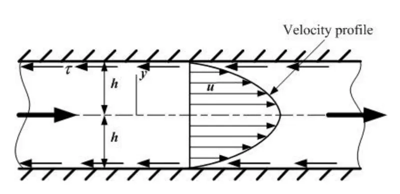
The image below depicts normal pipe flow for a pipe totally full with flowing fluid. Because of the no-slip condition, the velocity is greatest in the core of the pipe and zero at the solid surface.

Next let us Consider a fluid entering a circular pipe at uniform velocity,

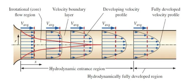
Because of the no-slip conditions along the pipe's walls, fluid particles that come into touch with the wall come to a full halt. As a result of the friction, the neighbouring layers of the fluid slow down as well. To compensate for the decrease in velocity, the fluid velocity at the pipe's midsection must rise in order to maintain a consistent mass flow rate down the pipe.

The following are the several areas of the pipe depicted in the above diagram:

1.The irrotational (core) flow area is one in which frictional effects are minor and the velocity in the radial direction is practically constant.

2.The velocity boundary layer is the area of flow where the effects of viscous shearing forces induced by fluid viscosity are felt and velocity fluctuations are considerable.

3.The hydrodynamic entrance zone is the area between the pipe inlet and the point at which the velocity profile is fully produced, and the length of this region is referred to as the hydrodynamic entry length.

4.Flow at the entry area is referred to as hydrodynamically developing flow because the velocity profile develops there. The hydrodynamically fully developed area is the region beyond the entry zone where the velocity profile is fully established and remains unchanging.

AXISYMMETRIC FLOW:

Axisymmetric flow refers to a type of fluid motion in which the properties of the flow remain unchanged when the flow is rotated about an axis. This axis is typically the central axis of a symmetric object, such as a cylinder or a cone. In other words, the flow field is invariant under rotation.In axisymmetric flow, the velocity and other flow parameters depend only on the radial distance from the axis of symmetry. This simplifies the analysis of fluid dynamics problems, as the governing equations can be expressed in terms of a single variable (radial distance) instead of multiple variables.

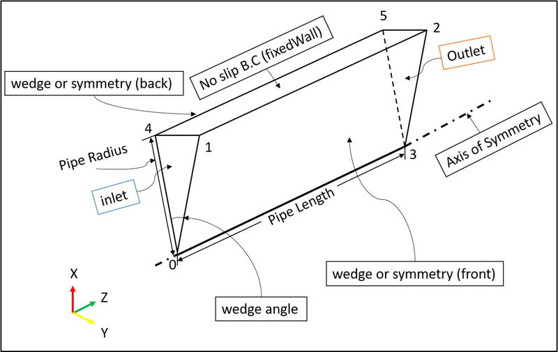
If our computers are not strong enough to conduct these simulations correctly, simulating flow through a cylinder may be expensive and computationally exhausting. So, for this, we will divide our domain and simulate only a portion of it (wedge) by utilising the axi-symmetric character of the flow and adding a symmetry boundary condition.

The wedge's cross section is depicted below.

Difference in Laminar and Turbulent Conditions:

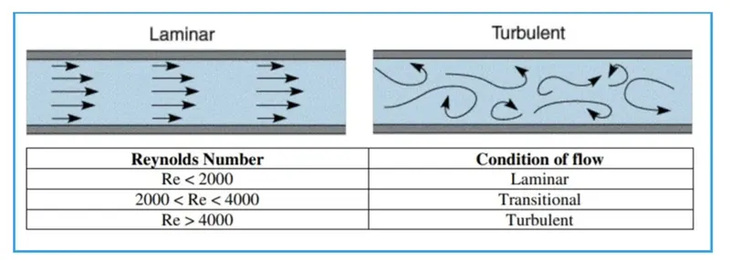
· The stream lines in laminar flow travel parallel to one other. With little or no mixing, the fluid particles travel in planes that glide over each other. There are no crosscurrents perpendicular to the flow direction, nor are there any eddies or swirls of fluid.

· When the velocity of flow in a pipe exceeds a certain threshold value for a specific fluid, the flow becomes turbulent. Turbulent flow is defined as flow that becomes erratically varying with time; the flow becomes unstable.

Reynolds number:

The Reynolds number, named after Osborne Reynolds, is a dimensionless quantity used in fluid mechanics to predict the flow patterns in different fluid flow situations. It is defined as the ratio of inertial forces to viscous forces within a fluid, and it plays a fundamental role in determining the type of flow regime a fluid will exhibit.

The formula for Reynolds number,

Re = ρ.v.L / m

Where,

ρ is the density of the fluid,

v is the velocity of the fluid,

L is a characteristic length (such as the diameter of a pipe),

μ is the dynamic viscosity of the fluid.

For flow through a circular pipe,

Hagen-Poiseuille's theory:

Hagen-Poiseuille's theory, named after Gotthilf Hagen and Jean Louis Marie Poiseuille, provides a fundamental understanding of laminar flow in long, straight pipes. The theory is particularly applicable to viscous, incompressible fluids like liquids. Here are the key points of Hagen-Poiseuille's theory:

Flow in a Pipe: The theory focuses on the steady, fully developed flow of an incompressible fluid through a cylindrical pipe of constant cross-sectional area.

Assumptions: Hagen-Poiseuille's theory makes several assumptions, including laminar flow, steady-state conditions, and negligible entrance effects. Laminar flow implies that the fluid flows in smooth, parallel layers without turbulence.

Application: Hagen-Poiseuille's theory is valuable in understanding fluid flow in small-diameter tubes, capillaries, and blood vessels. It has applications in fields such as physiology, medicine, and engineering.

Limitations: The theory is limited to laminar flows and does not account for turbulence. In real-world situations, especially in larger pipes or when flow rates are high, turbulent effects may become significant, and the theory may not accurately predict the flow behaviour.

The pressure drop in an incompressible and Newtonian fluid in laminar flow through a long cylindrical pipe of constant cross – section can be derived as,

Δp = 8μVLR2 = 32μVLD2

Where,

Δp= Pressure difference between the two ends (p1–p2)

L = Length of the pipe

μ = Dynamic viscosity

V = Velocity of Fluid

R= Pipe radius

D = Pipe Diameter.

The ratio of length to radius of a pipe should be greater than one forty-eighth of the Reynolds number for the Hagen–Poiseuille law to be valid. If the pipe is too short, the Hagen–Poiseuille equation may result in unphysically high flow rates.

A few examples in which the Hagen–Poiseuille law is practically applied is the air flow in lung alveoli, or the flow through a drinking straw or through a hypodermic needle. It is also applied for the process of blood flow through a narrow constriction.

EQUATIONS AND CALCULATIONS :

We are considering the working fluid flowing inside the cross section of the pipe to be water at an ambient temperature of 25ºC

Given Data :

Geometry of the flow is axi - symmetric.

The flow is laminar and flows through a constant cross section.

Inlet Reynold’s Number, Re=2100

Wedge angle should be less than 5º.

Analytical Solution :

Diameter of the pipe

D=0.02m → R=D2=0.01 m

Density of working fluid (water) at 25°C

ρ=997 kgm3

Wedge angle

θ=4°

Dynamic Viscosity of water at 25°C

μ=8.90×10−4

Kinematic Viscosity of water at 25°C

ν=μρ

= 8.90×10−4997

ν 8.92×10−7 m2sec

Hydrodynamic Entrance Length

Lh=0.06⋅Re⋅D

=0.06×2100×0.02

Lh=2.52

Total Length of the Pipe

L=2.8

Average Velocity

Vavg=μ⋅Reρ⋅D

=8.90×10−4 × 2100997×0.02

Vavg=0.0937

Maximum Velocity

Vmax=2⋅Vavg

=2×0.0937

Vmax=0.1874

Velocity Profile

u(r)=2⋅Vavg⋅(1–r2R2)

Pressure Drop

Δp = 32⋅μ⋅Vavg⋅LD2

=32×8.90×10−4×0.0937×2.8(0.02)2

Δp=18.680 Pa

Kinematic Pressure Drop

Kinematic Δp=Δpρ

=18.680997

Kinematic Δp=0.0187

Procedure:

Setup:

We begin by browsing to the tutorials directory of OpenFOAM using the "tut" command in the terminal window. We must use the tutorials to determine the best case file for our given problem, which is axi-symmetric laminar flow over a constant cross section pipe. The "ls" command is used to list the contents (files or directories) of a directory.

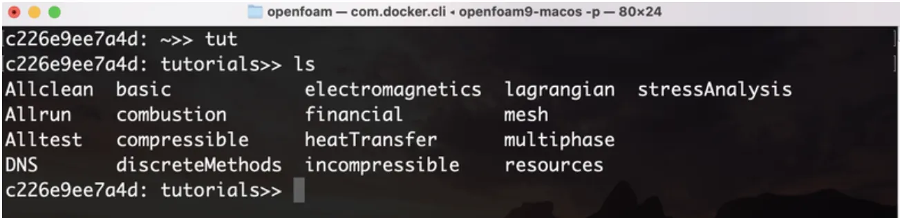
We browse into the incompressible directory since it is an incompressible flow. To traverse and modify the working directory in the terminal window, we use the "cd" command.

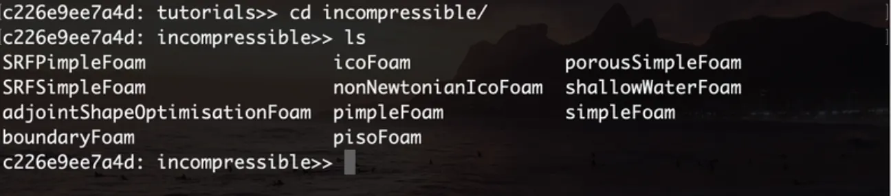
The next step is to navigate to the icoFoam directory, as this problem's solver type is icoFoam. The incompressible laminar Navier-Stokes equations are solved with the icoFoam programme. Because the code is inherently transient, it necessitates a starting condition (such as zero velocity) and boundary conditions.

To establish our needed domain, we utilise the cavity utility. We transfer this directory into the $FOAM_RUN file, which OpenFOAM produces by default. We use the "cp -r" command to recursively transfer the contents of the file or directory into the $FOAM_RUN folder as "Flow Through Pipe" for personal usage. We make a duplicate of the files because OpenFOAM does not allow us to edit or update its built-in instructional files.

CODE FILE:

% SIMULATION OF FLOW THROUGH A PIPE
% Code to automate generation of blockMeshDict file
clear all
close all
clc


% INPUTS
% Assumptions
% Diameter of Pipe (m)
D = 0.02; 

% Radius of Pipe (m)
R = D/2;

% Reynold's Number
Re = 2100;

% Wedge Angle (degrees)
theta = 4;

% Total Length of the Pipe (m)
L = 2.8;



% Assuming working fluid is water at 25° C
% Density of water (kg/m³)
rho = 997;

% Dynamic Viscosity of Water (Pa.s)
mu = 8.90 * 10^-4;

% Kinematic Viscosity of Water (m^2/s)
nu = mu/rho;


% Hydrodynamic Entrance Length (m)
L_h = 0.06 * Re * D;



% HAGEN - POISEUILLE'S FLOW EQUATIONS
% Average Velocity (m/s)
V_avg = (mu * Re)/(rho * D);

% Maximum Velocity (m/s)
V_max = 2 * V_avg;

% Pressure Drop (Pa)
delta_p = (32*mu*V_avg*L)/(D^2);

% Kinematic Pressure Drop (Pa)
kinematic_delta_p = delta_p/rho;



% DEFINING THE GEOMETRY
% Vertices
V0 = [0 0 0];
V1 = [0 R*cosd(theta/2) -R*sind(theta/2)];
V2 = [0 R*cosd(theta/2) R*sind(theta/2)];

V3 = [L 0 0];
V4 = [L R*cosd(theta/2) -R*sind(theta/2)];
V5 = [L R*cosd(theta/2) R*sind(theta/2)];




% BLOCKMESHDICT FILE
% Creating the file
% Header
h1 = '/*--------------------------------*- C++ -*----------------------------------*\';
h2 = '  =========                 |';
h3 = '  \\      /  F ield         | OpenFOAM: The Open Source CFD Toolbox';
h4 = '   \\    /   O peration     | Website:  https://openfoam.org';
h5 = '    \\  /    A nd           | Version:  9';
h6 = '     \\/     M anipulation  |';
h7 = '\*---------------------------------------------------------------------------*/';
h8 = 'FoamFile';
h9 = '{';
h10 = '    format      ascii;';
h11 = '    class       dictionary;';
h12 = '    object      blockMeshDict;';
h13 = '}';
h14 = '// * * * * * * * * * * * * * * * * * * * * * * * * * * * * * * * * * * * * * //';


% Creating BlockMesh File
f1 = fopen('blockMeshDict.txt','w');

% Header
fprintf(f1,'%s\n',h1);
fprintf(f1,'%s\n',h2);
fprintf(f1,'%s\n',h3);
fprintf(f1,'%s\n',h4);
fprintf(f1,'%s\n',h5);
fprintf(f1,'%s\n',h6);
fprintf(f1,'%s\n',h7);
fprintf(f1,'%s\n',h8);
fprintf(f1,'%s\n',h9);
fprintf(f1,'%s\n',h10);
fprintf(f1,'%s\n',h11);
fprintf(f1,'%s\n',h12);
fprintf(f1,'%s\n',h13);
fprintf(f1,'%s\n\n',h14);

% Conversion Factor
fprintf(f1,'%s\n\n','convertToMeters 1;');

% Vertices
fprintf(f1,'%s\n','vertices');
fprintf(f1,'%s\n','(');
fprintf(f1,'\t(%d %d %d)\n',V0);
fprintf(f1,'\t(%d %f %f)\n',V1);
fprintf(f1,'\t(%d %f %f)\n',V2);
fprintf(f1,'\t(%.2f %d %d)\n',V3);
fprintf(f1,'\t(%.2f %f %f)\n',V4);
fprintf(f1,'\t(%.2f %f %f)\n',V5);
fprintf(f1,'%s\n\n',');');

% Blocks
fprintf(f1,'%s\n','blocks');
fprintf(f1,'%s\n','(');
fprintf(f1,'\thex (0 3 4 1 0 3 5 2) (400 30 1) simpleGrading (1 0.1 1)\n');
fprintf(f1,'%s\n\n',');');

% Edges
fprintf(f1,'%s\n','edges');
fprintf(f1,'%s\n','(');
fprintf(f1,'\tarc 2 1 (%d %.3f %d)\n',0,R,0);
fprintf(f1,'\tarc 5 4 (%.3f %.3f %d)\n',L,R,0);
fprintf(f1,'%s\n\n',');');

% Boundary
fprintf(f1,'%s\n','boundary');
fprintf(f1,'%s\n','(');

% Axis
fprintf(f1,'\taxis\n');
fprintf(f1,'\t{\n');
fprintf(f1,'\t\ttype empty;\n');
fprintf(f1,'\t\tfaces\n');
fprintf(f1,'\t\t(\n');
fprintf(f1,'\t\t\t(0 3 3 0)\n');
fprintf(f1,'\t\t);\n');
fprintf(f1,'\t}\n\n');

% Inlet
fprintf(f1,'\tinlet\n');
fprintf(f1,'\t{\n');
fprintf(f1,'\t\ttype patch;\n');
fprintf(f1,'\t\tfaces\n');
fprintf(f1,'\t\t(\n');
fprintf(f1,'\t\t\t(0 1 2 0)\n');
fprintf(f1,'\t\t);\n');
fprintf(f1,'\t}\n\n');

% Outlet
fprintf(f1,'\toutlet\n');
fprintf(f1,'\t{\n');
fprintf(f1,'\t\ttype patch;\n');
fprintf(f1,'\t\tfaces\n');
fprintf(f1,'\t\t(\n');
fprintf(f1,'\t\t\t(3 5 4 3)\n');
fprintf(f1,'\t\t);\n');
fprintf(f1,'\t}\n\n');

% Front Face
fprintf(f1,'\tfront\n');
fprintf(f1,'\t{\n');
fprintf(f1,'\t\ttype wedge;\n');
fprintf(f1,'\t\tfaces\n');
fprintf(f1,'\t\t(\n');
fprintf(f1,'\t\t\t(0 3 4 1)\n');
fprintf(f1,'\t\t);\n');
fprintf(f1,'\t}\n\n');

% Back Face
fprintf(f1,'\tback\n');
fprintf(f1,'\t{\n');
fprintf(f1,'\t\ttype wedge;\n');
fprintf(f1,'\t\tfaces\n');
fprintf(f1,'\t\t(\n');
fprintf(f1,'\t\t\t(0 2 5 3)\n');
fprintf(f1,'\t\t);\n');
fprintf(f1,'\t}\n\n');

% Top Wall
fprintf(f1,'\tpipeWall\n');
fprintf(f1,'\t{\n');
fprintf(f1,'\t\ttype wall;\n');
fprintf(f1,'\t\tfaces\n');
fprintf(f1,'\t\t(\n');
fprintf(f1,'\t\t\t(1 4 5 2)\n');
fprintf(f1,'\t\t);\n');
fprintf(f1,'\t}\n');

fprintf(f1,'%s\n\n',');');
fprintf(f1,'%s\n','mergePatchPairs');
fprintf(f1,'%s\n','(');
fprintf(f1,'%s\n\n',');');
fprintf(f1,'%s\n','// ************************************************************************* //');

We get our respective blockMeshDict file from the above code.

1.The vertices of the wedge are constructed by computing the values of Rcos(2) and Rsin(2) with regard to the wedge's axis.

2.In the code, we use the "fprintf" command to write the contents of the file, resulting in the blockMeshDict text file shown below.

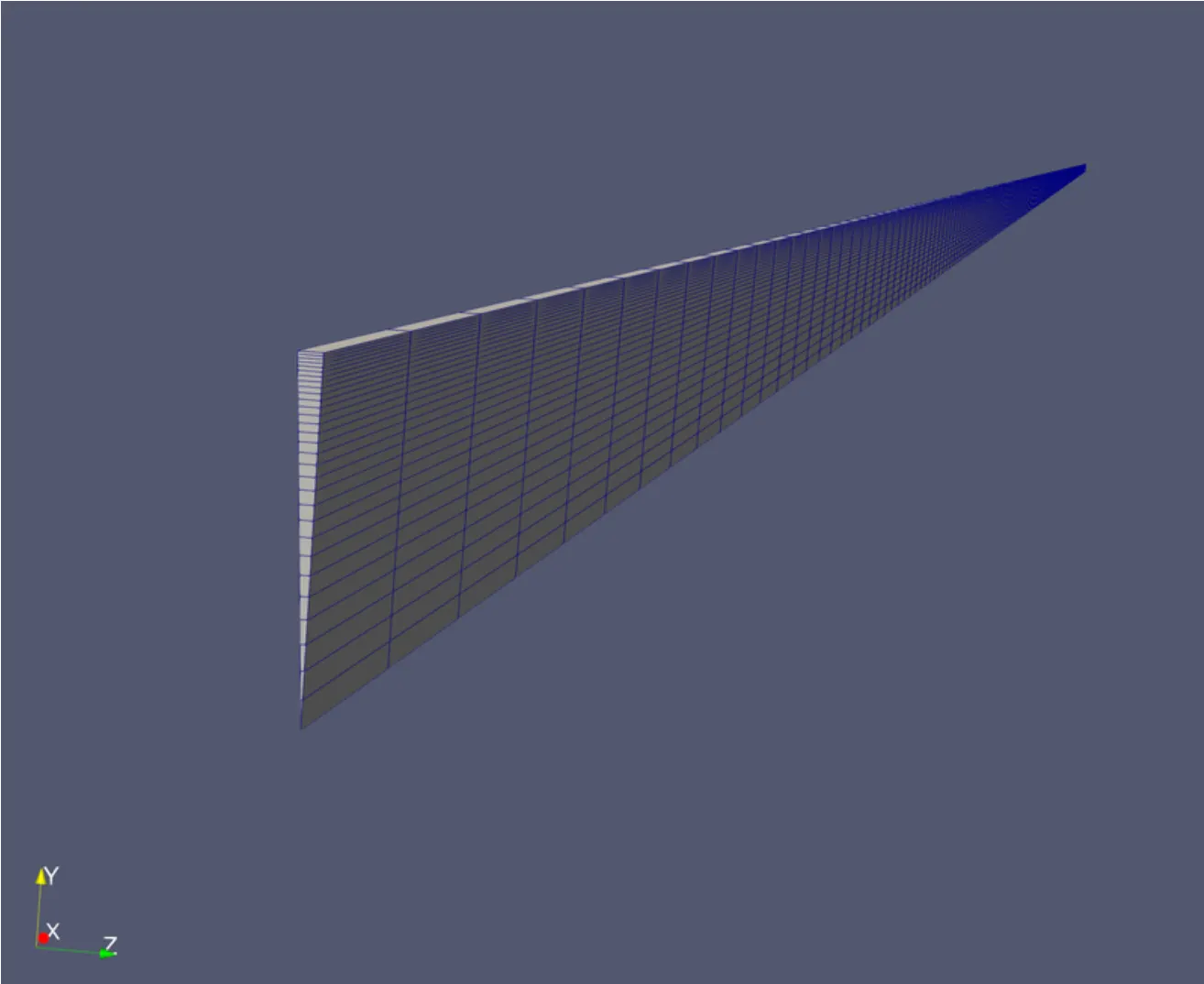
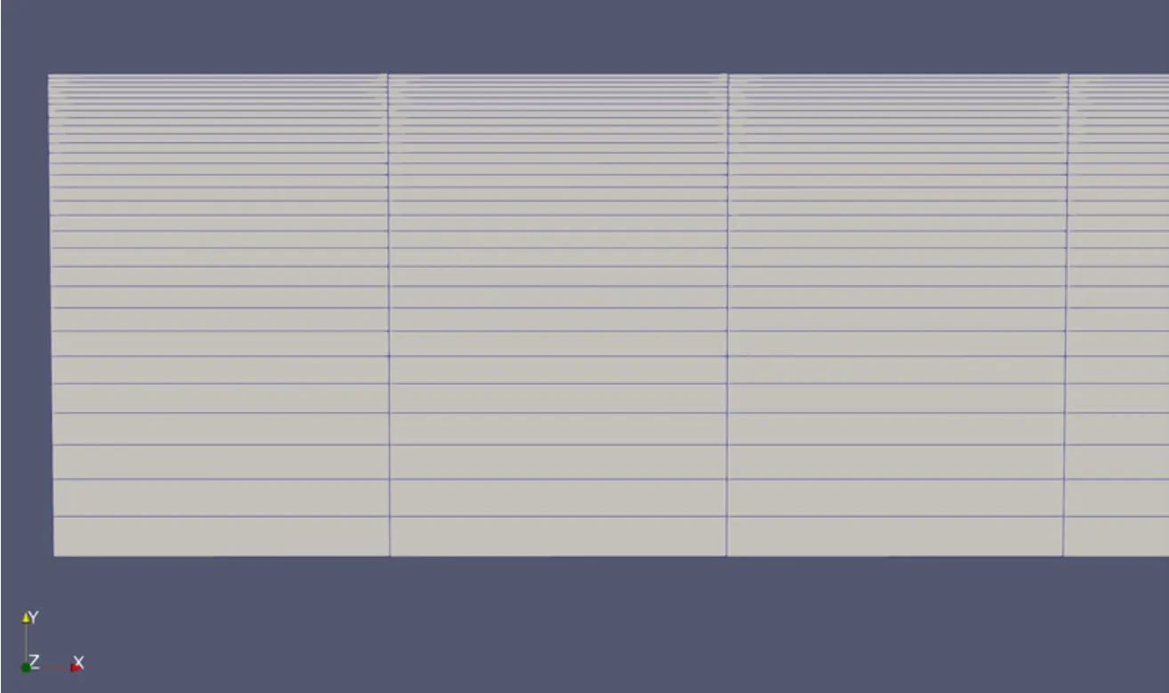
3.Using the estimated vertices, we generate the wedge geometry using the hexahedral mesh. For this simulation, we employ a grading factor of 0.1 to get finer meshing along the walls.

4.The number of cells on the x, y, and z axes is 400, 30, and 1, respectively.

We create an arc representing the radius of the wedge and also define the input, output, axis, wall, front and back faces of the wedge.

blockMeshDict File :

X/*--------------------------------*- C++ -*----------------------------------*\
  =========                 |
  \\      /  F ield         | OpenFOAM: The Open Source CFD Toolbox
   \\    /   O peration     | Website:  https://openfoam.org
    \\  /    A nd           | Version:  9
     \\/     M anipulation  |
\*---------------------------------------------------------------------------*/
FoamFile
{
    format      ascii;
    class       dictionary;
    object      blockMeshDict;
}
// * * * * * * * * * * * * * * * * * * * * * * * * * * * * * * * * * * * * * //

convertToMeters 1;

vertices
(
	(0 0 0)
	(0 0.009994 -0.000349)
	(0 0.009994 0.000349)
	(2.80 0 0)
	(2.80 0.009994 -0.000349)
	(2.80 0.009994 0.000349)
);

blocks
(
	hex (0 3 4 1 0 3 5 2) (400 30 1) simpleGrading (1 0.1 1)
);

edges
(
	arc 2 1 (0 0.010 0)
	arc 5 4 (2.800 0.010 0)
);

boundary
(
	axis
	{
		type empty;
		faces
		(
			(0 3 3 0)
		);
	}

	inlet
	{
		type patch;
		faces
		(
			(0 1 2 0)
		);
	}

	outlet
	{
		type patch;
		faces
		(
			(3 5 4 3)
		);
	}

	front
	{
		type wedge;
		faces
		(
			(0 3 4 1)
		);
	}

	back
	{
		type wedge;
		faces
		(
			(0 2 5 3)
		);
	}

	pipeWall
	{
		type wall;
		faces
		(
			(1 4 5 2)
		);
	}
);

mergePatchPairs
(
);

// ************************************************************************* //

We get our respective blockMeshDict file from the above code.

Controldict file:

/*--------------------------------*- C++ -*----------------------------------*\
  =========                 |
  \\      /  F ield         | OpenFOAM: The Open Source CFD Toolbox
   \\    /   O peration     | Website:  https://openfoam.org
    \\  /    A nd           | Version:  9
     \\/     M anipulation  |
\*---------------------------------------------------------------------------*/
FoamFile
{
    format      ascii;
    class       dictionary;
    location    "system";
    object      controlDict;
}
// * * * * * * * * * * * * * * * * * * * * * * * * * * * * * * * * * * * * * //

application     icoFoam;

startFrom       startTime;

startTime       0;

stopAt          endTime;

endTime         40;

deltaT          0.01;

writeControl    timeStep;

writeInterval   200;

purgeWrite      0;

writeFormat     ascii;

writePrecision  6;

writeCompression off;

timeFormat      general;

timePrecision   6;

runTimeModifiable true;


// ************************************************************************* //

Transport property file:

/*--------------------------------*- C++ -*----------------------------------*\
  =========                 |
  \\      /  F ield         | OpenFOAM: The Open Source CFD Toolbox
   \\    /   O peration     | Website:  https://openfoam.org
    \\  /    A nd           | Version:  9
     \\/     M anipulation  |
\*---------------------------------------------------------------------------*/
FoamFile
{
    format      ascii;
    class       dictionary;
    location    "constant";
    object      transportProperties;
}
// * * * * * * * * * * * * * * * * * * * * * * * * * * * * * * * * * * * * * //

nu              [0 2 -1 0 0 0 0] 8.9268e-07;


// ************************************************************************* //

Velocity file:

/*--------------------------------*- C++ -*----------------------------------*\
  =========                 |
  \\      /  F ield         | OpenFOAM: The Open Source CFD Toolbox
   \\    /   O peration     | Website:  https://openfoam.org
    \\  /    A nd           | Version:  9
     \\/     M anipulation  |
\*---------------------------------------------------------------------------*/
FoamFile
{
    format      ascii;
    class       volVectorField;
    object      U;
}
// * * * * * * * * * * * * * * * * * * * * * * * * * * * * * * * * * * * * * //

dimensions      [0 1 -1 0 0 0 0];

internalField   uniform (0.0937 0 0);

boundaryField
{
    axis
    {
        type            empty;
    }
    
    inlet
    {
        type            fixedValue;
        value           uniform (0.0937 0 0);
    }
    
    outlet
    {
        type            zeroGradient;
    }

    front
    {
        type            wedge;
    }

    back
    {
        type            wedge;
    }
    
    pipeWall
    {
        type            noSlip;
    }
}

// ************************************************************************* //

Pressure file:

/*--------------------------------*- C++ -*----------------------------------*\
  =========                 |
  \\      /  F ield         | OpenFOAM: The Open Source CFD Toolbox
   \\    /   O peration     | Website:  https://openfoam.org
    \\  /    A nd           | Version:  9
     \\/     M anipulation  |
\*---------------------------------------------------------------------------*/
FoamFile
{
    format      ascii;
    class       volScalarField;
    object      p;
}
// * * * * * * * * * * * * * * * * * * * * * * * * * * * * * * * * * * * * * //

dimensions      [0 2 -2 0 0 0 0];

internalField   uniform 0;

boundaryField
{
    axis
    {
        type            empty;
    }
    
    inlet
    {
        type            zeroGradient;
    }
    
    outlet
    {
        type            zeroGradient;
        value           uniform 0.0187;
    }

    front
    {
        type            wedge;
    }

    back
    {
        type            wedge;
    }
    
    pipeWall
    {
        type            zeroGradient;
    }
}

// ************************************************************************* //

RESULTS :

By running the simulation with the above mentioned data, we get the outputs as follows,

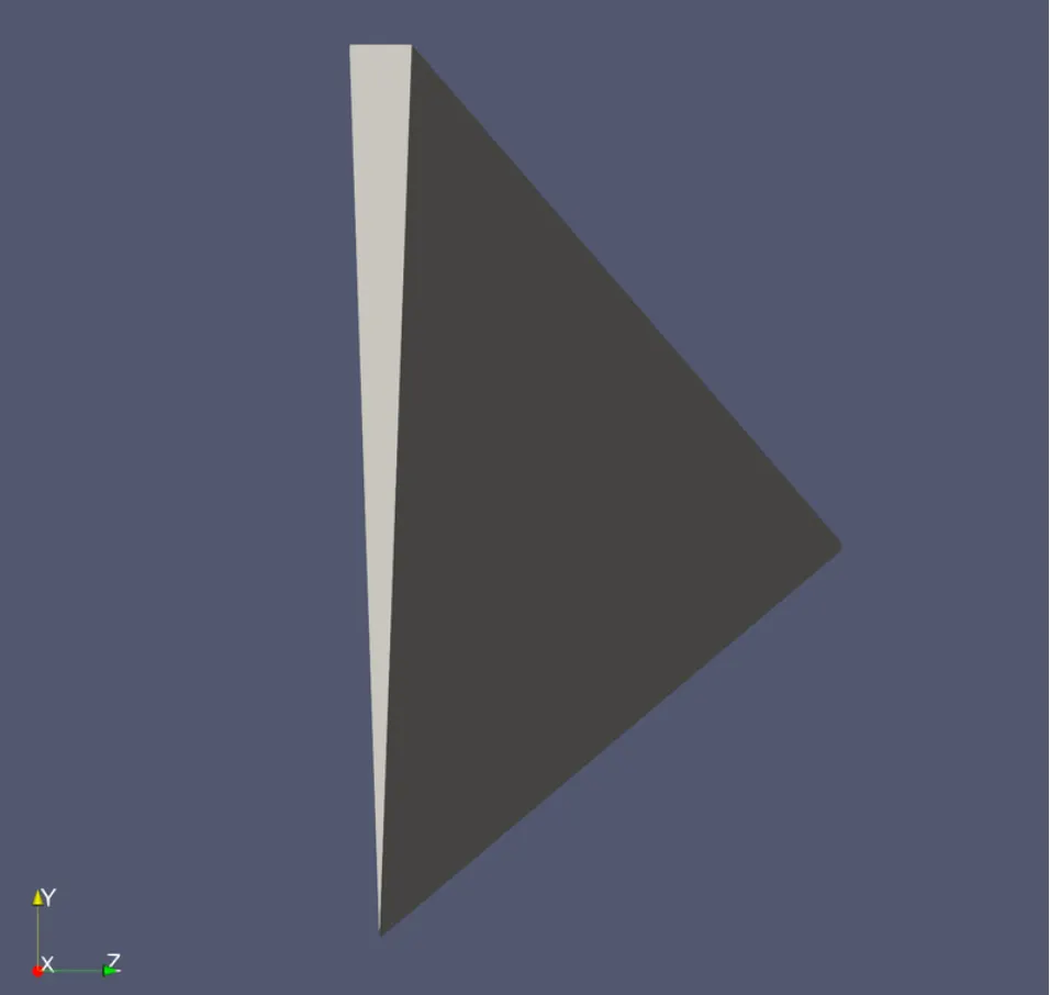
1.WEDGE

We create a cross section of the pipe, i.e; a wedge geometry, with a wedge angle of 4o as shown below.

Geometry :

Meshing (axi - symmetric) :

2.VELOCITY PROFILES

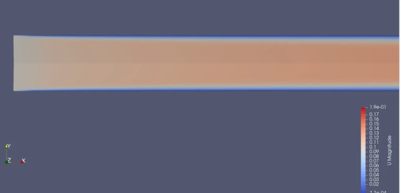
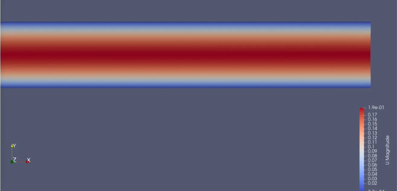
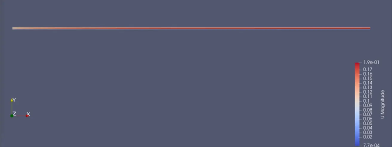
The change in velocity of the fluid flowing inside the wedge section is as shown below.

At inlet :

outlet:

velocity distribution:

https://drive.google.com/file/d/1jk2QVvfTdJ0w8NLMszYq4mnkXerg5vrW/view?usp=sharing

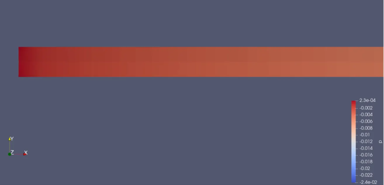
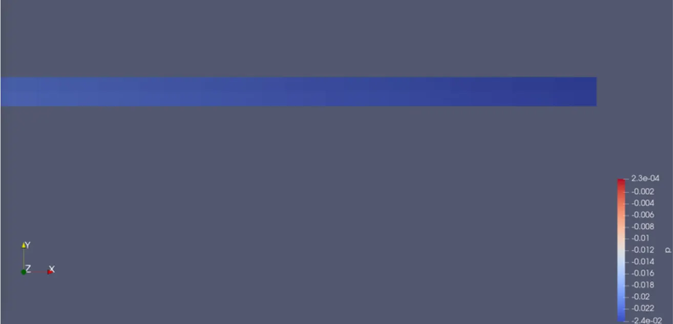
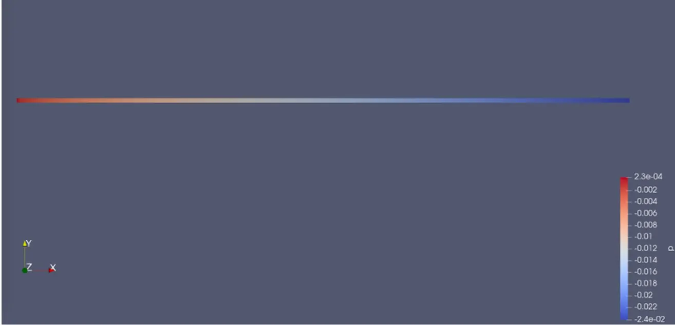
3.PRESSURE PROFILES

The pressure distribution across the cross sectional pipe is represented as follows.

At inlet :

outlet:

pressure distribution:

https://drive.google.com/file/d/1WWGcD4qS2qz1CHB0c3v1SYe_Tx20zRrT/view?usp=sharing

Graphs:

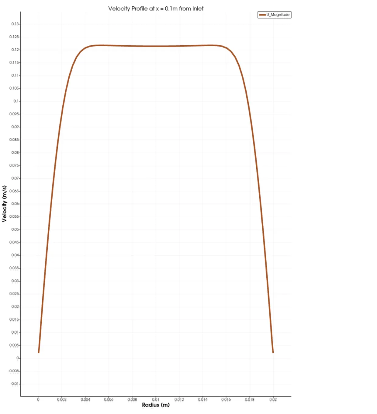
1. velocity profiles:

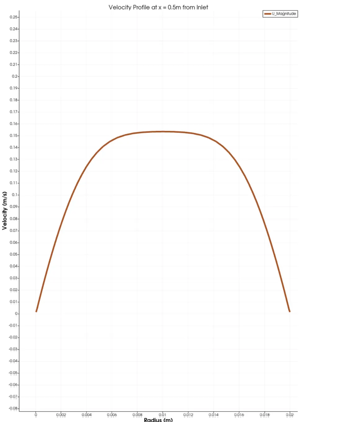
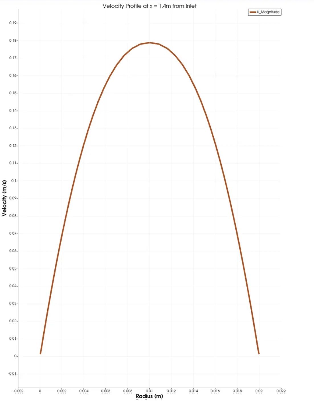
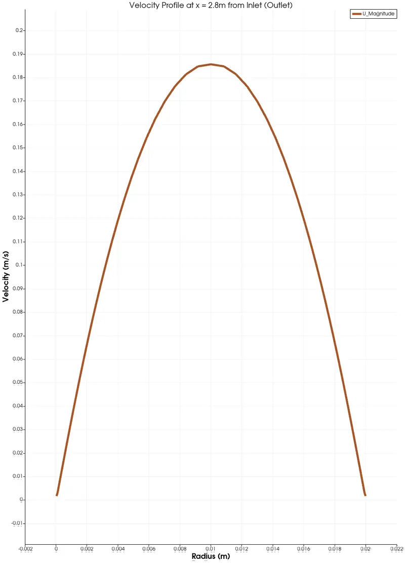
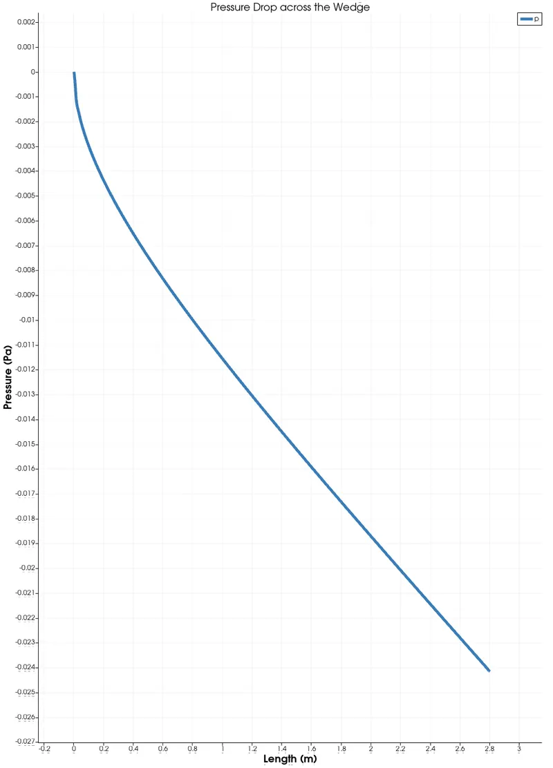
2. pressure drop:

ANALYSIS OF SHEAR STRESS:

Shear strains form when the fluid is in motion due to the particles in the fluid moving relative to one another. Shear stress can produce a shift in fluid flow between layers depending on the material.

For a fluid flowing in a pipe, fluid velocity will be zero at the pipe wall. Velocity will increase while moving towards the centre of the pipe. Shear forces are normally present because adjacent layers of the fluid move with different velocities compared to each other.

The formula for shear stress for a fluid is given by,

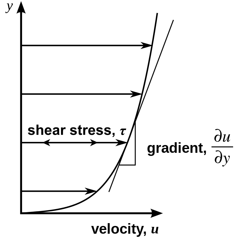
Where,

μ= Dynamic Viscosity (Pa.s)

τ= Shear Stress = FA

F = Applied Force

A= Cross-sectional area parallel to the direction of the applied force

∂u/∂v = Rate of Shear Deformation (Shear Rate)

Results and discussion:

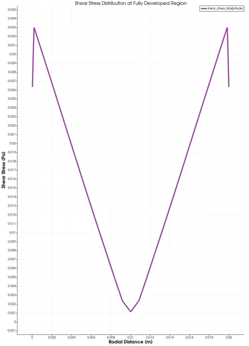
Final plot,

1.Using the wedge boundary condition over a constant cross section pipe with an intake Reynolds number of 2100 and a wedge angle of 4°, we successfully simulated an axi - symmetric flow.

2.We can see from the charts that the fluid velocity at the pipe walls remains zero due to the no-slip boundary constraint we specified. We can also see that as the distance from the intake rises, the velocity profiles gradually form and get sharper (parabolic).

3.Based on the pressure graphs acquired from the simulation, we can see that the fluid pressure is highest at the intake of the pipe and progressively declines along its length. We can observe that the pressure is lowest near the exit, hence the pressure drop derived from this simulation follows the Hagen - Poiseuille's Theory.

4.Shear stresses form in the fluid as a result of the relative motion of the fluid layers next to the pipe walls, which have a no - slip boundary condition, resulting in zero velocity at the pipe walls. We can see from the shear stress plot that shear stresses are greatest at the pipe's walls and gradually drop as they approach the pipe's core, as the relative friction between the layers reduces.

5.We acquire our individual wedge shape and velocity profiles from the simulation run, as illustrated above. We conduct a test to investigate the flow characteristics at various locations of the pipe in order to evaluate the velocity profiles. We investigate the velocity profile plots in four locations of the pipe, at distances of 1m, 0.5m, 1.4m, and 2.8m (outlet) from the pipe's intake.

Week 10 - Simulation of Flow through a pipe in OpenFoam

Ship work like this
in your own course.

Talk to a career counsellor

Ship work like thisin your own course.

Talk to a career counsellor

Ship work like this
in your own course.