Week 5.1 - Mid term project - Solving the steady and unsteady 2D heat conduction problem

Aim:

To solve the 2D heat conduction equation under steady and transient conditions using the both explicit and implicit methods.

Objective:   

1. Steady state analysis & Transient State Analysis

To Solve the 2D heat conduction equation by using the point iterative techniques that were taught in the class. The Boundary conditions for the problem, The Boundary conditions for the problem are as follows;

Top Boundary = 600 K

Bottom Boundary = 900 K

Left Boundary = 400 K

Right Boundary = 800 K

You will implement the following methods for solving implicit equations.

• Jacobi
• Gauss-seidel
• Successive over-relaxation

Your absolute error criteria is 1e-4

2. You will write code for both implicit and explicit schemes 

3. Compare the convergence rate [Number of iterations] of the steady state and transient [explicit and implicit] simulations and justify the numerics.

Overview:

Heat conduction (or thermal conduction) is the transfer of heat from one item to another with a different temperature when they come into direct contact. In this project, we will use explicit and implicit methods to solve the 2D heat conduction equation under steady and transient circumstances. The heat equation is a second order partial differential equation that describes how the distribution of a quantity such as heat changes over time in a solid medium as it flows spontaneously from higher to lower points. It is a subset of the diffusion equation.

It is more common in physics and engineering contexts, particularly in the context of diffusion over a medium, to fix a Cartesian coordinate system and then investigate the specific situation of a function T(x, y, z, t) having three spatial variables (x, y, z) and time variable t. Then, u is said to be a solution of the heat equation.

     

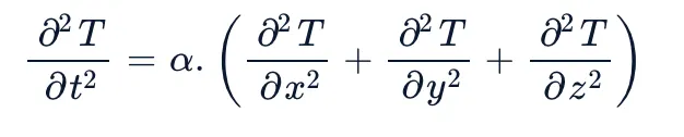
Let us see about the various theories,

Discretization:
         Discretization methods are used to split a continuous function's area, i.e., the real solution to a system of differential equations, into a discrete function, where the solution values are determined at each point in space and time. Discretization simply refers to the spacing between each point in solution space, followed by the substitution of difference quotients for derivatives in the governing equation.

Steady state:

        Steady-state means that the qualities measured in any field of space do not change over time. In general, the qualities of a given point of interest do not change and stay constant throughout the procedure, even after some time(t). This is the fundamental idea behind a steady-state system. So, when a system is said to be in a steady-state condition, it is providing a better case to fix the assumption values, which makes the calculation better. This concept is also widely used in engineering problems, and when we see it applied in the domain of heat transfer, our region of interest would be in determining the heat transfer across the field to determine its temperature profile. 

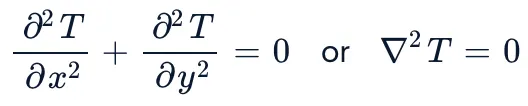
The Steady State form of the 2-D Heat Conduction Equation is given by,(Laplacian Equation),

Finite Difference Method:
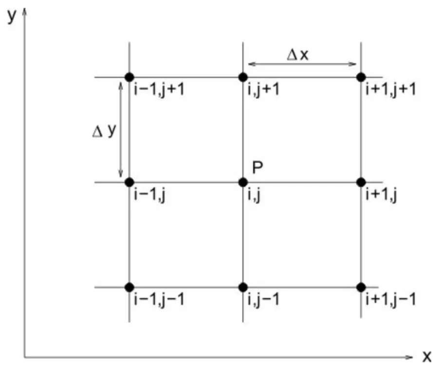
          Finite-difference methods (FDM) are a set of numerical techniques used in numerical analysis to solve differential equations by approximating derivatives using finite differences. It provides numerical solutions for values at discrete places in the domain known as grid points based on finite differences.

To compute approximate derivatives, the finite differences approach is utilised. This is used in numerical analysis to solve numerical ordinary differential equations and numerical partial differential equations. The methods that arise are known as finite-difference methods. Taylor series expansions are used to generate finite difference representations of derivatives.

Iterative Point Technique:
             An iterative technique generates a succession of improved approximate solutions for a class of problems from a starting value, with the n-th approximation generated from the preceding ones. An iterative method algorithm is a precise implementation of an iterative technique, including the termination criteria. If the associated sequence converges for given starting approximations, an iterative process is said to be convergent.

Unsteady State (Transient State):
                    Heat transfer is the process through which heat energy flows from an elevated temperature source to a lower temperature side. Conduction, convection, and radiation are the other mechanisms of heat transport, and we will only discuss conduction here. Any system that experiences a change in energy inside itself as a result of temperature difference begins in an unsteady state condition, where the temperature change happens with regard to time. 

This is because there will be a large temperature difference between the system and its surroundings at the start of the process, causing it to adapt an unsteady or transient condition of heat transfer at first, but once the inlet energy flow and the energy going out (which causes the transient condition) become equal, there will only be steady-state heat transfer prevailing inside the system until the temperature reaches a steady-state. 

The equation is given by,

The Implicit Method:

            When a calculation is performed for a dependent variable, a set of equations and a matrix are used to identify the unknown variable. This is known as the Implicit approach. Because this method uses simultaneous equations and uses guess values as the initial values to find the approximated values, it is unconditionally stable. As a result, no stability criteria are required to obtain stable results, and the computational time required for the solution to converge is high. The computation time is reduced when the estimate values are closer to the target value. Because no stability conditions are required, greater time steps can be employed.

The Explicit Method:

             When an unknown quantity is directly computed in terms of a known quantity. This calculation is known as Explicit. This approach necessitates the application of stability criteria, which, when met, results in a stable solution. Because of the stability criterion, tiny time steps are required to achieve stable solutions. The number of computations rises as the time step decreases, hence the computing time required for the solution to converge decreases while the accuracy of the answer increases.

We can solve the Linear equations in CFD in two methods namely,

•  Direct method
• Iterative method. 

The Direct Method:
           The direct technique solves a (n x n) matrix with a fixed number of steps by combining Gauss-Seidel and Jacobian methods. However, this approach is inefficient for some engineering issues since they may include millions of cells making a massive matrix to solve. As a result, the system needs demand additional space to solve such a large matrix. As a result, using the Direct Method to solve linear equations in CFD is not a viable option.Therefore, we take a different approach to solving such equations, namely iterative methods.

The Iterative Method:
          Iterative techniques are a superior and more efficient alternative to the Direct approach. Here, we will solve the equations in such a way that the previously calculated values for a specific grid point at its corresponding time step (for transient conditions only) or from its previous time step are used to calculate the function at that specific point using the reframed governing equations that follow the criterion of different iterative solvers, such as,

• Jacobian Iterative Solver
• Gauss-Seidel Iterative Solver
• Successive Over Relaxation Iterative Solver  

Let us see in detail about the following,

1.The Jacobian Iterative Solver

The Jacobian Iterative Solver is a numerical technique used to solve systems of nonlinear equations. It's particularly valuable when linear methods are insufficient due to the nonlinearity of the equations. The solver employs an iterative approach by iteratively refining the solution based on linear approximations derived from the Jacobian matrix, which contains partial derivatives of the equations with respect to the variables. In each iteration, the solver computes a correction to the current solution using the Jacobian matrix and updates the solution accordingly. The process continues until a convergence criterion is met. The Jacobian Iterative Solver finds applications in various scientific, engineering, and mathematical fields, where complex nonlinear relationships need to be analyzed and solved numerically.

2.The Gauss-Seidel Iterative Solver

The Gauss-Seidel Iterative Solver is a numerical method used to solve systems of linear equations iteratively. It's an extension of the Jacobi method and is particularly suited for solving sparse linear systems, where only a few coefficients in each equation are nonzero.The Gauss-Seidel Iterative Solver can converge faster than the Jacobi method because it utilizes updated values as soon as they become available. However, its convergence depends on the properties of the coefficient matrix A, and it may not converge for all matrices. It's commonly used when dealing with systems arising from finite difference or finite element discretization, and it's especially effective for diagonally dominant matrices.

3.Successive Over Relaxation Iterative Solver  

The Successive Over Relaxation Iterative Solver is a numerical technique used to solve systems of linear equations iteratively, particularly when the coefficient matrix is diagonally dominant or positive definite. SOR is an extension of the Gauss-Seidel method and incorporates a relaxation factor to accelerate convergence.The SOR Iterative Solver is particularly effective for diagonally dominant or positive definite matrices. The choice of the relaxation factor ω is crucial, if ω is selected optimally, convergence can be accelerated. However, choosing an inappropriate ω might hinder convergence.

2D heat conduction equation

The two-dimensional steady-state heat conduction equation is a fundamental equation in heat transfer and thermal analysis. It describes the distribution of temperature in a two-dimensional region over time when the system has reached a state where temperature changes are not occurring.

The equation is typically written as:

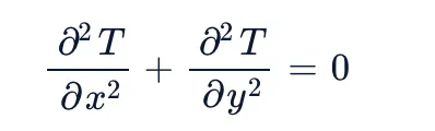
where:

•  is the temperature at any point (x,y) in the two-dimensional region.
• ​ ∂2T/∂x2 represents the second partial derivative of T with respect to x, describing how temperature changes with respect to the x-direction.
• ∂2T/∂y2​ represents the second partial derivative of T with respect to y, describing how temperature changes with respect to the y-direction.

To apply the Central Difference technique for space derivative, discretize this second order partial differential equation in space along (x & y axis). For space, the partial derivative can be approximated using the derivative definition.

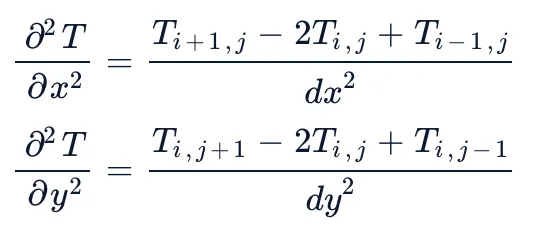
By substituting the above equation in steady state 2D heat conduction equation,

and we get,

Let us simplify the equation further by,

• T_(i,j)    = T_P
• T_(i+1,j) = T_R
• T_(i-1,j) = T_L
• T_(i,j+1) = T_T
• T_(i,j-1) = T_B

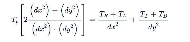
And finally we get,

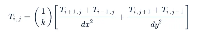
The Jacobian Iterative Solver

The Gauss-Seidel Iterative Solver

Successive Over Relaxation Iterative Solver  

Transient state analysis of 2D heat equation :

The transient equation is,

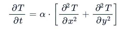
To discretize this equation in space and time, utilise the Forward Difference scheme for time derivative and the Central Difference strategy for space derivative. The derivative definition will be used to approximate the partial derivative in both space and time.
 we take ,

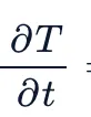as Time derivative term,

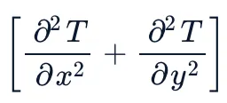as Space derivative term,

α as Thermal diffusity.

Time derivative:

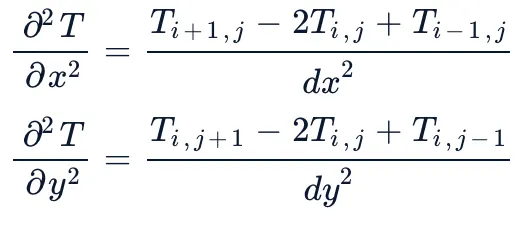
Substituting above equation,

finally we can get,

This equation is used in program to solve the 2-D Heat conduction equation numerically. 

Now we will see about the Explicit And Implicit Method:

1.Explicit Method:

In an explicit method, the value of the dependent variable at the next time step is calculated using information solely from the current time step. This calculation is "explicit" because the formula directly expresses the new value in terms of known quantities at the current time step. Explicit methods are generally easier to implement and computationally less demanding than implicit methods, but they might have limitations in terms of stability and accuracy.

The Explicit equation:

2.Implicit Method:

In an implicit method, the value of the dependent variable at the next time step is calculated using information from both the current and future time steps. The calculation is "implicit" because the formula involves an equation that relates the future value to itself and other quantities, requiring a solution for the new value. Implicit methods are often more stable and accurate than explicit methods but might require solving equations iteratively or analytically, which can be computationally more intensive.

The Implicit equation:

Let us see the MATLAB codings i used,

The Function Code:

% Creating a function to solve Iterative Methods,

function [T,iteration]=Iterative_solver(tol,error,It_s,nx,ny,T_old,T,dx,dy,k)

  iteration=0;

   switch It_s     % Switching to Iterative Methods

       %% Solving Using Jacobi Method,

       case 1

     while(error>tol)           % Convergence loop    

               for i=2:nx-1     % Spacial loop on x

                   for j=2:ny-1 % spacial loop on y

                       H=(T_old(i-1,j)+T_old(i+1,j))/(dx^2);

                       V=(T_old(i,j-1)+T_old(i,j+1))/(dy^2);

                       T(i,j)=k*(H+V);

                  end

              end

          error=max(max(abs(T-T_old)));

          T_old=T;    % Updating Temperature

          iteration=iteration+1;

     end

      %% Solving Using Gauss Seidal method,

     case 2

     while(error>tol)           % Convergence loop    

               for i=2:nx-1     % Spacial loop on x

                   for j=2:ny-1 % spacial loop on y

                      H=(T(i-1,j)+T_old(i+1,j))/(dx^2);

                      V=(T(i,j-1)+T_old(i,j+1))/(dy^2);

                      T(i,j)=k*(H+V);

                  end

              end

          error=max(max(abs(T-T_old)));

          T_old=T;   % Updating Temperature

          iteration=iteration+1;

     end

     %% Solving Using Successive Over Relaxation Method (SOR),

     case 3

     omega=1.5;

     while(error>tol)           % Convergence loop    

               for i=2:nx-1     % Spacial loop on x

                   for j=2:ny-1 % spacial loop on y

                      H=(T(i-1,j)+T_old(i+1,j))/(dx^2);

                      V=(T(i,j-1)+T_old(i,j+1))/(dy^2);

                      T(i,j)=k*(H+V);

                      T(i,j)=T_old(i,j)*(1-omega)+(omega*T(i,j));

                  end

              end

          error=max(max(abs(T-T_old)));

          T_old=T;   % Updating Temperature

          iteration=iteration+1;        

     end

   end

end

Main code:

%% Solving 2-D Temperature Heat Conduction Equation,

% Steady State Heat Conduction Equation,

clear all;close all;clc

%% Inputting the parameters for Domain,

l=1;      % Length of the domain

nx=40;    % Number of Nodes on X -Axis

ny=nx;    % Number of Nodes on y -Axis

�fining the length of domain repect to number of nodes,

x=linspace(0,l,nx);

y=linspace(0,l,ny);

% Finding the Grid Size along x and y axis,

dx=x(2)-x(1);  % Along X-axis

dy=y(2)-y(1);  % Along Y-axis

%�fining the Temperature,

T_i=250;    % Initial condition for Temperature

T=T_i*ones(nx,ny);

% Applying Boundary Conditions,

T_L=400;     

T_T=600;

T_R=800;

T_B=900;

% Assigning Boundary Conditions on Nodes,

T(1,:)=600;      % Temperature on Top

T(end,:)=900;    % Temperature on Bottom

T(:,1)=400;      % Temperature on Left

T(:,end)=800;    % Temperature on Right

% Assigning Average Temperature on Corner Grids,

T(1,1)=(T_L+T_T)/2;

T(1,ny)=(T_R+T_T)/2;

T(nx,1)=(T_L+T_B)/2;

T(nx,ny)=(T_B+T_R)/2;

% Updating the Temperature,

T_old=T;

�fining Error & Tolerance;

tol=1e-4;   % Tolerence

error=1e5;  % Error

It_s=1:3;   % For Different Iterative Schemes (Jcobo - 1, Gauss Seidal- 2, SOR - 3)

�lculation

k=(dx^2*dy^2)/(2*(dx^2+dy^2));

%�lling a function to solve Iterative Solvers,

[T_J,iteration_jacobi]=Iterative_solver(tol,error,It_s(1),nx,ny,T_old,T,dx,dy,k);  �lling Jacobi Method

[T_GS,iteration_GS]=Iterative_solver(tol,error,It_s(2),nx,ny,T_old,T,dx,dy,k);     �lling Gauss Seidal Method

[T_SOR,iteration_SOR]=Iterative_solver(tol,error,It_s(3),nx,ny,T_old,T,dx,dy,k);   �lling SOR Method

%% Plotting,

% Plotting for Temperature Distribution by Jacobi Method

figure("Name",'STEADY STATE ANALYSIS')

contourf(x,y,T_J,'ShowText','on','LineWidth',0.5);

colorbar

colormap(jet)

set(gca,'YDir','reverse')

text_title=({'2-DSteady State Heat Conduction (Jacobi Method)';['No.of.Grid Points =',num2str(nx)];['Total Iterations =',num2str(iteration_jacobi)]});

title(text_title)

xlabel('X-Direction')

ylabel('Y-Direction')

% Plotting for Temperature Distribution by Gauss Seidal Method

figure("Name",'STEADY STATE ANALYSIS')

contourf(x,y,T_GS,'ShowText','on','LineWidth',0.5);

colorbar

colormap(jet)

set(gca,'YDir','reverse')

text_title=({'2-D Steady State Heat Conduction (Gauss Seidal Method)';['No.of.Grid Points =',num2str(nx)];['Total Iterations =',num2str(iteration_GS)]});

title(text_title)

xlabel('X-Direction')

ylabel('Y-Direction')

% Plotting for Temperature Distribution by Successive Over Relaxation (SOR) Method

figure("Name",'STEADY STATE ANALYSIS')

contourf(x,y,T_SOR,'ShowText','on','LineWidth',0.5);

colorbar

colormap(jet)

set(gca,'YDir','reverse')

text_title=({'2-D Steady State Heat Conduction (SOR Method)';['No.of.Grid Points =',num2str(nx)];['Total Iterations =',num2str(iteration_SOR)]});

title(text_title)

xlabel('X-Direction')

ylabel('Y-Direction')

Code explanation:

1. Input Parameters: The code starts by initializing parameters like domain length, number of nodes on the x and y axes, and initial conditions.

2. Grid Generation: The domain is discretized into a grid by creating vectors for x and y values using the 'linspace' function. The grid size (dx and dy) is calculated.

3. Temperature Initialization: The initial temperature field is set uniformly to a value T_i

4. Boundary Conditions: Boundary temperatures (TL​, TT​, TR​, TB​) are defined. Then, boundary temperatures are applied to the corresponding nodes in the temperature matrix T.

5. Corner Averaging: The average temperature of corner nodes is calculated by averaging adjacent boundary temperatures and assigning it to the corner nodes.

6. Iterative Solver: The code calls the 'Iterative_solver' function for each iterative method (Jacobi, Gauss-Seidel, and SOR) with specified tolerances, error, and parameters.

7. Plotting: The temperature distributions obtained from each method are plotted using 'contourf' to visualize the results. The 'colormap' function defines the color map for the contour plots.

The code then proceeds to plot the temperature distributions obtained from each iterative method separately using the 'contourf' function, setting titles, labels, and other formatting options to enhance visualization.

Transient state heat conduction:

EXPLICT:

%% Solving 2-D Temperature Heat Conduction Equation,

% Transient Heat Conduction Equation, By Using Explicit Method,

clear all;close all;clc

% Inputting the parameters for Domain,

l=1;      % Length of the domain

nx=40;    % Number of Nodes on X -Axis

ny=nx;    % Number of Nodes on y -Axis

�fining the length of domain repect to number of nodes,

x=linspace(0,l,nx);   % Along X-Direction

y=linspace(0,l,ny);   % Along Y- Direction

% Finding the Grid Size along x and y axis,

dx=x(2)-x(1);

dy=y(2)-y(1);

�fining the Initial Temperature,

T_i=250;           % Initial condition for Temperature

T=T_i*ones(nx,ny); % Assigning Temperature on nodes

% Applying Boundary Conditions,

T_L=400;        % Temperature on the Left

T_T=600;        % Temperature on the TOP

T_R=800;        % Temperature on the RIGHT

T_B=900;        % Temperature on the BOTTOM

% Assigning Boundary Conditions on Nodes,

T(1,:)=600;      % Temperature on Top

T(end,:)=900;    % Temperature on Bottom

T(:,1)=400;      % Temperature on Left

T(:,end)=800;    % Temperature on Right

% Assigning Average Temperature on Corner Grids,

T(1,1)=(T_L+T_T)/2;

T(1,ny)=(T_R+T_T)/2;

T(nx,1)=(T_L+T_B)/2;

T(nx,ny)=(T_B+T_R)/2;

% Updating the current Temperature,

T_old=T;

�fining the Time Steps

t=0.15;     % Time for Temperature Distribution

dt=1e-4;    % Time steps

nt=t/dt;    % Number of Time Steps

alpha=1.4;  % Thermal Diffusivity

�lculations,

k1=alpha*(dt/dx^2);

k2=alpha*(dt/dy^2);

CFL=k1+k2;

%% TIME MARCHING PROCEDURE,

   Iteration=1;

   for k=1:nt    % Time loop

        for i=2:nx-1      % Space loop

            for j=2:ny-1  % Space loop

                H=(T_old(i+1,j)-2*T(i,j)+T_old(i-1,j));

                V=(T_old(i,j+1)-2*T(i,j)+T_old(i,j-1));

                T(i,j)=T_old(i,j)+k1*(H)+k2*(V);

            end

        end

        T_old=T;

        Iteration=Iteration+1;

   end

%% PLOTTING FOR EXPLICIT METHOD

figure('Name','TRANSIENT STATE ANALYSIS - EXPLICIT')

contourf(x,y,T,'ShowText','on','LineWidth',0.5);

colorbar

colormap(jet)

set(gca,'YDir','reverse')

title('2-D Transient State Heat Conduction (Explicit Method)')

text=sprintf(['Total Iterations =%d;  ','CFL=%g\n   ','Grid Points=%g;  ','dt=%g;  ','dx=%g'],...

              Iteration,CFL,nx,dt,dx);

subtitle(text)

xlabel('X-Direction')

ylabel('Y-Direction')

Code explanation:

1. input Parameters: The code initializes parameters such as the domain length, number of nodes on the x and y axes, and the initial temperature.

2. Grid Generation: The domain is discretized into a grid using the 'linspace' function, and the grid size (dx and dy) is calculated.

3. Initial Temperature: The initial temperature field is set uniformly to a value T_i.

4. Boundary Conditions: Boundary temperatures (TL​, TT​, TR​, TB​) are defined, and they are applied to the corresponding nodes in the temperature matrix T.

5. Corner Averaging: The average temperature of corner nodes is calculated by averaging adjacent boundary temperatures and assigning it to the corner nodes.

6. Time Step Definition: The total time 't' for the simulation is defined, along with the time step 'dt'. The number of time steps nt is calculated based on the total time and time step.

7. Thermal Diffusivity Calculation: The coefficient k1 and k2 are calculated based on thermal diffusivity (α) and grid parameters.

8. Time Marching Loop: The main time marching loop iterates through time steps ('k' for time) and space nodes ('i' and 'j' for x and y directions).

9. Updating Temperature: The temperature at each interior node is updated using the explicit method. The Laplacian operator (H and V) approximations are calculated using the temperature at previous time step 'T_old'.

10. Boundary Temperature Retention: The boundary temperatures are not updated during each time step.

11. Plotting: After completing the time marching loop, the temperature distribution is plotted using 'contourf'. The plot shows the changing temperature distribution over time. 

IMPLICIT:

%% Solving 2-Dimensional Temperature Heat Conduction Equation,

% Transient Heat Conduction Equation, By Using Implicit Method,

clear all;close all;clc

%% Inputting the Domain Parmeters,

l=1;      % Length of the domain

nx=40;    % Number of Nodes on X -Axis

ny=nx;    % Number of Nodes on y -Axis

�fining the length of domain repect to number of nodes,

x=linspace(0,l,nx);

y=linspace(0,l,ny);

% Finding the Grid Size along x and y axis,

dx=x(2)-x(1);   % On X-axis

dy=y(2)-y(1);   % on Y-axis

%�fining the Initial Temperature,

T_i=250;           % Initial condition for Temperature

T=T_i*ones(nx,ny); % Assigning Temperature on nodes

% Applying Boundary Conditions,

T_L=400;        % Temperature on the Left

T_T=600;        % Temperature on the TOP

T_R=800;        % Temperature on the RIGHT

T_B=900;        % Temperature on the BOTTOM

% Assigning Boundary Conditions on Nodes,

T(1,:)=600;      % Temperature on Top

T(end,:)=900;    % Temperature on Bottom

T(:,1)=400;      % Temperature on Left

T(:,end)=800;    % Temperature on Right

% Assigning Average Temperature on Corner Grids,

T(1,1)=(T_L+T_T)/2;

T(1,ny)=(T_R+T_T)/2;

T(nx,1)=(T_L+T_B)/2;

T(nx,ny)=(T_B+T_R)/2;

% Updating the Temperatures,

T_old=T;

T_prev=T;

�fining the Time Steps

t=0.2;     % Time for Temperature Distribution

dt=1e-4;    % Time steps

nt=t/dt;    % Number of Time Steps

alpha=1.4;  % Thermal Diffusivity

�lculations,

k1=alpha*(dt/dx^2);

k2=alpha*(dt/dy^2);

CFL=k1+k2;

Term1=1/(1+(2*(k1+k2)));

Term2=k1*Term1;

Term3=k2*Term1;

�fining the Tolerence,

tol=1e-4;     % Tolerence Creteria

omega=1.2;    % Relaxation Factor

Iteration=1;  % Initial Iteration

%% Input User Selection Prompt,

prompt=(['Select Iterative Method\n (1).JACOBI ITERATIVE METHOD\n ' ...

    '(2).GAUSS SEIDAL ITERATIVE METHOD\n ' ...

    '(3).SOR ITERATIVE METHOD\n']);

Iterative_Method=input(prompt);

%% Solving 2-D Using Iterative Method,

% Time loop,

tic

for k=1:nt

   error=1e5;     % Initialize Error on each iteration time loop

   if Iterative_Method==1    %% Jacobi Iterative Method

    % Convergence loop

    while error>tol

        % Nodal loop

        for i=2:nx-1

            for j=2:ny-1

                 H=(T_old(i+1,j)+T_old(i-1,j));

                 V=(T_old(i,j+1)+T_old(i,j-1));

                 T(i,j)=((T_prev(i,j)*Term1)+(Term2*H)+(Term3*V));

            end

        end

        error=max(max(abs(T-T_old)));

        % Updating temperatures,

        T_old=T;

        Iteration=Iteration+1;

    end

  end

%% Gauss Seidal Iterative Method

if Iterative_Method==2   

    % Convergence loop

    while error>tol

        % Nodal loop

        for i=2:nx-1

            for j=2:ny-1

                 H=(T_old(i+1,j)+T(i-1,j));

                 V=(T_old(i,j+1)+T(i,j-1));

                 T(i,j)=((T_prev(i,j)*Term1)+(Term2*H)+(Term3*V));

            end

        end

        error=max(max(abs(T-T_old)));

        % Updating temperatures,

        T_old=T;

        Iteration=Iteration+1;

    end

end

%% Successive Over Relaxation (SOR) Iterative Method

   if Iterative_Method==3

    % Convergence loop

    while error>tol

        % Nodal loop

        for i=2:nx-1

            for j=2:ny-1

                 H=(T(i-1,j)+T_old(i+1,j));

                 V=(T(i,j-1)+T_old(i,j+1));

                 T(i,j)=((T_prev(i,j)*Term1)+(Term2*H)+(Term3*V));

                 T(i,j)=(T_old(i,j)*(1-omega))+omega*T(i,j);

            end

        end

        error=max(max(abs(T-T_old)));

        % Updating temperatures,

        T_old=T;

        Iteration=Iteration+1;

    end

   end

    T_prev=T;

    sim_time_Jacobi=toc;   % Simulation time for Jacobi Iteration

    sim_time_Gs=toc;       % Simulation time for Gauss seidal Iteration

    sim_time_SOR=toc;      % Simulation time for SOR Iteration

%% Plotting

figure(1)

contourf(x,y,T,'ShowText','on','LineWidth',0.5)

colorbar

colormap('jet')

set(gca,'YDir','reverse')

    if Iterative_Method==1

    title('2-D Transient State Heat Conduction (Implicit - Jacobi Method)')

    text=sprintf(['Total Iterations =%d;  ','CFL=%g\n   ','Grid Points=%g;  ','dt=%g;  ','dx=%g\n','Simulation Time=%g'],...

                  Iteration,CFL,nx,dt,dx,sim_time_Jacobi);

    subtitle(text)

    elseif Iterative_Method==2

    title('2-D Transient State Heat Conduction (Implicit - Gauss Seidal Method)')

    text=sprintf(['Total Iterations =%d;  ','CFL=%g\n   ','Grid Points=%g;  ','dt=%g;  ','dx=%g\n','Simulation Time=%g'],...

                  Iteration,CFL,nx,dt,dx,sim_time_Gs);

    subtitle(text)

    elseif Iterative_Method==3

    title('2-D Transient State Heat Conduction (Implicit - SOR Method)')

    text=sprintf(['Total Iterations =%d;  ','CFL=%g\n   ','Grid Points=%g;  ','dt=%g;  ','dx=%g\n','Simulation Time=%g'],...

                  Iteration,CFL,nx,dt,dx,sim_time_SOR);

    subtitle(text)

    end

xlabel('X-Direction')

ylabel('Y-Direction')

end

Code explanation:

1. Input Parameters: The code initializes parameters such as the domain length, number of nodes on the x and y axes, and initial conditions.

2. Grid Generation: The domain is discretized into a grid using the 'linspace' function, and the grid size (dx and dy) is calculated.

3. Initial Temperature: The initial temperature field is set uniformly to a value 'T_i'.

4. Boundary Conditions: Boundary temperatures (TL​, TT​, TR​, TB​) are defined, and they are applied to the corresponding nodes in the temperature matrix T.

5. Corner Averaging: The average temperature of corner nodes is calculated by averaging adjacent boundary temperatures and assigning it to the corner nodes.

6. Time Step Definition: The total time 't' for the simulation is defined, along with the time step 'dt'. The number of time steps 'nt' is calculated based on the total time and time step.

7. Thermal Diffusivity Calculation: The coefficients k1 and k2 are calculated based on thermal diffusivity (α) and grid parameters. The Courant-Friedrichs-Lewy (CFL) number is calculated.

8. Coefficient Terms: The terms 'Term1' ,  'Term2' ,  and 'Term3' are calculated for the implicit method.

9. User Input for Iterative Method: The code prompts the user to select an iterative method (1 for Jacobi, 2 for Gauss-Seidel, 3 for SOR).

10. Iterative Loop: The main time loop iterates through time steps (k) for the chosen iterative method. Within the time loop, an error convergence loop is employed to iteratively update the temperature distribution.

11. Updating Temperature: Depending on the selected iterative method, the temperature at each interior node is updated using the implicit method with the coefficients calculated earlier. The 'while' loop continues until the error falls below a specified tolerance.

12. Plotting: After each time loop iteration, the temperature distribution is plotted using 'contourf'. The plot title, subtitles, and labels are set based on the chosen iterative method and other relevant information.

13. Simulation Time Calculation: The simulation time is recorded for each iterative method using the 'tic and 'toc' functions.

Results and conclusion:

Steady state Heat conduction,

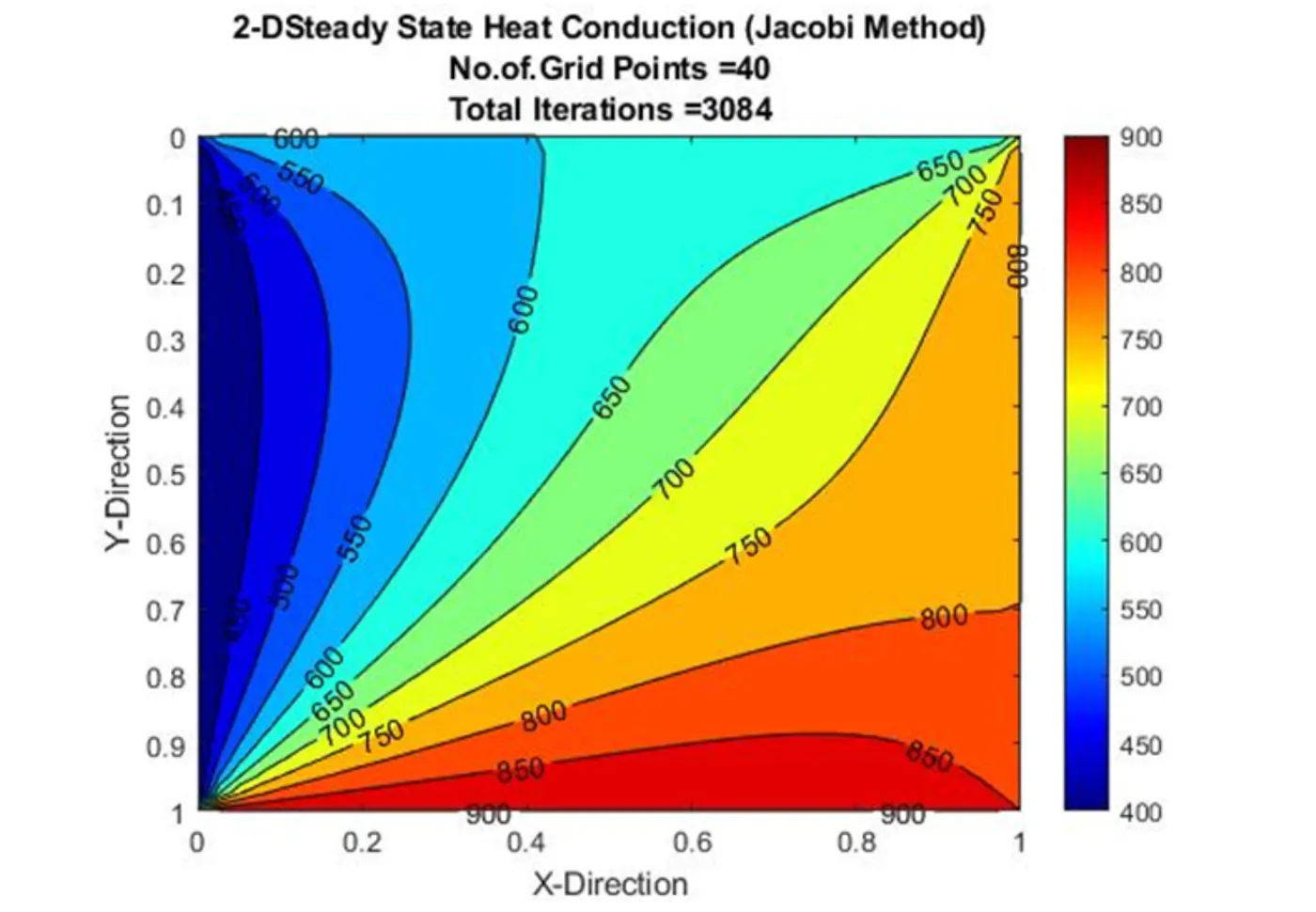
1.The plot depicts the temperature distribution along the x and y axes for the steady-state analysis of the 2-D heat conduction equation.
2.By graphing the temperature at the domain's bottom, the greater temperature may be disseminated around the domain.
3.The Jacobi Iterative approach is used for steady state analysis, and 3084 iterations are required to achieve steady state convergence for the domain.

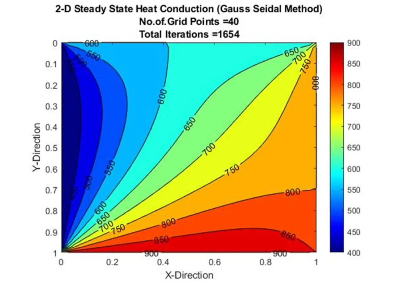
1.The plot depicts the temperature distribution along the x and y axes for the steady-state analysis of the 2-D heat conduction equation.
2.The temperature at the bottom of the domain can be dispersed throughout the x and y co-ordinates of a domain by graphing it.
3.The Gauss seidal Iterative technique is used for steady state analysis, and 1654 iterations are required to achieve steady state convergence for the domain.
The gauss seidal approach converges quicker than the Jacobi method.

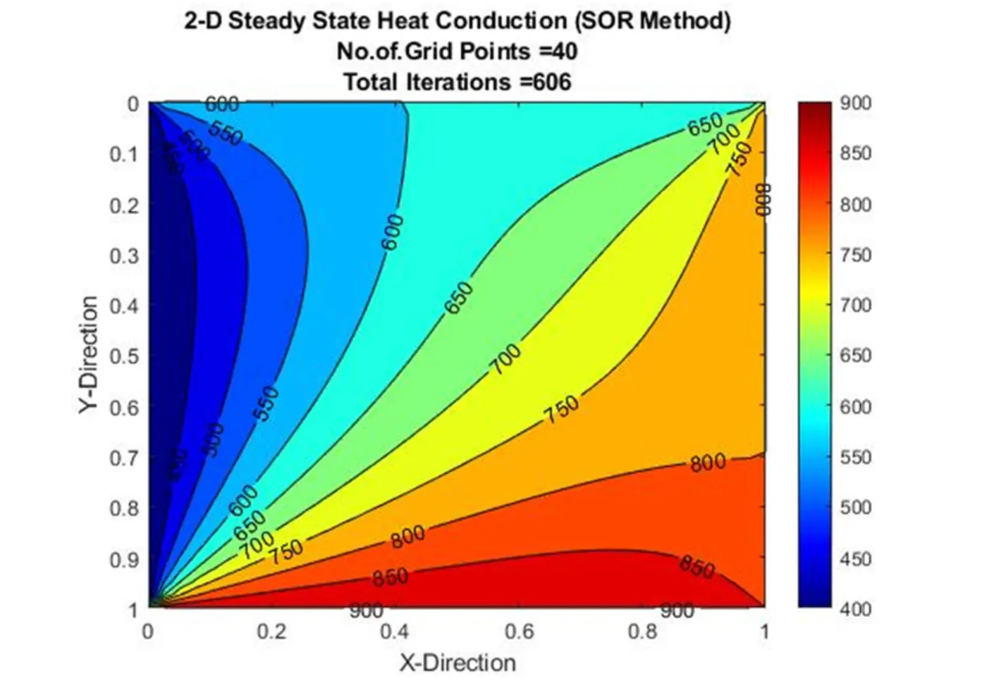
1.The plot depicts the temperature distribution along the x and y axes for the steady-state analysis of the 2-D heat conduction equation.
2.The temperature at the bottom of the domain can be dispersed throughout the x and y co-ordinates of a domain by graphing it.
3.The steady state analysis is done using the successive over relaxation iterative approach, and 606 iterations are required to achieve steady state convergence for the domain.
SOR iterative approach converges quicker than Jacobi method and Gauss seidal method.

Transient state:

Explicit,

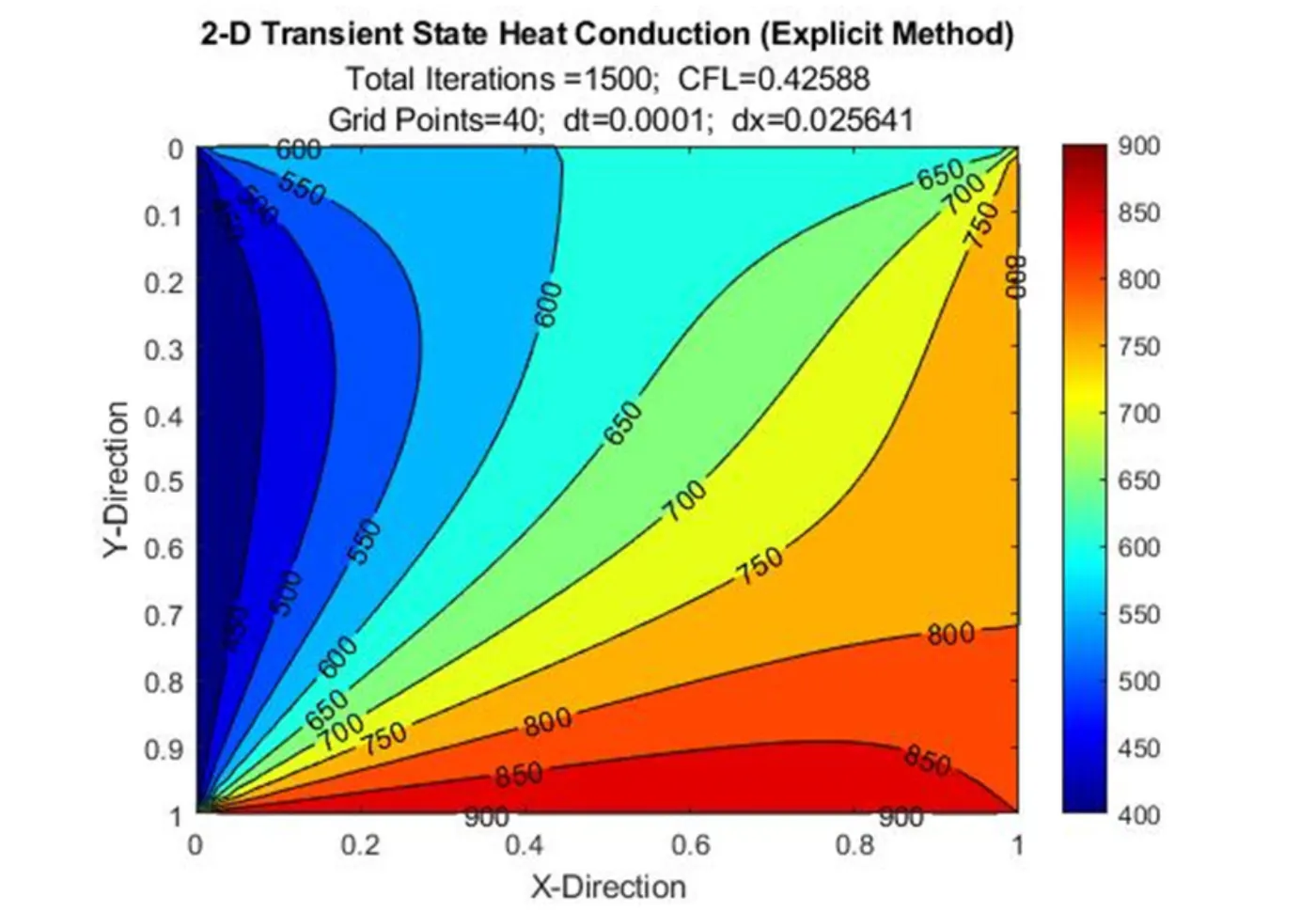
1.The plot depicts the temperature distribution along the x and y axes for the 2-D heat conduction equation's transient state analysis.
2.The temperature at the bottom of the domain can be dispersed throughout the x and y co-ordinates of a domain by graphing it.
3.The explicit technique is used for transient state analysis, and 1500 iterations are done to get steady-state convergence for the domain @ time step of 1e-4 @ dx= 0.02564.
4.The CFL requirements for the Explicit approach are critical to the solution's stability.
5.If the CFL values surpass 0.5, the solution will be unstable at that time step.

Implicit,

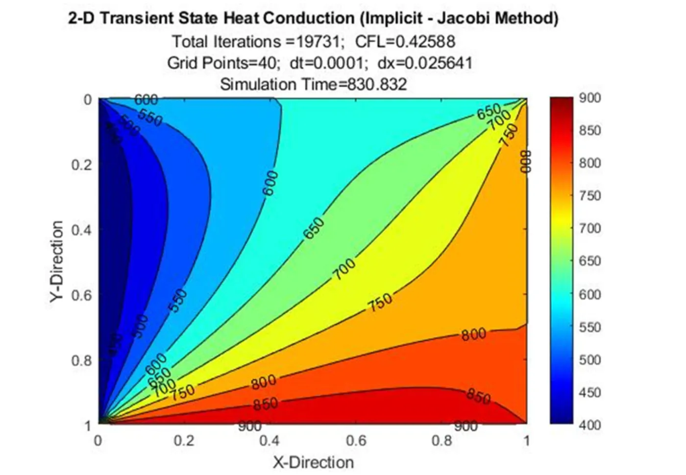
1.The plot implicitly represents the temperature distribution along the x and y axes for the transient state analysis of the 2-D heat conduction equation.
2.By graphing the temperature at the domain's bottom, the greater temperature may be disseminated around the domain.
3.The Jacobi Iterative approach is used for transient state analysis, and 19732 iterations are required to achieve steady-state convergence for the domain.
4.The convergence loop is executed within the time loop "nt," where the older temperature value and prior time step temperature values are updated correspondingly.

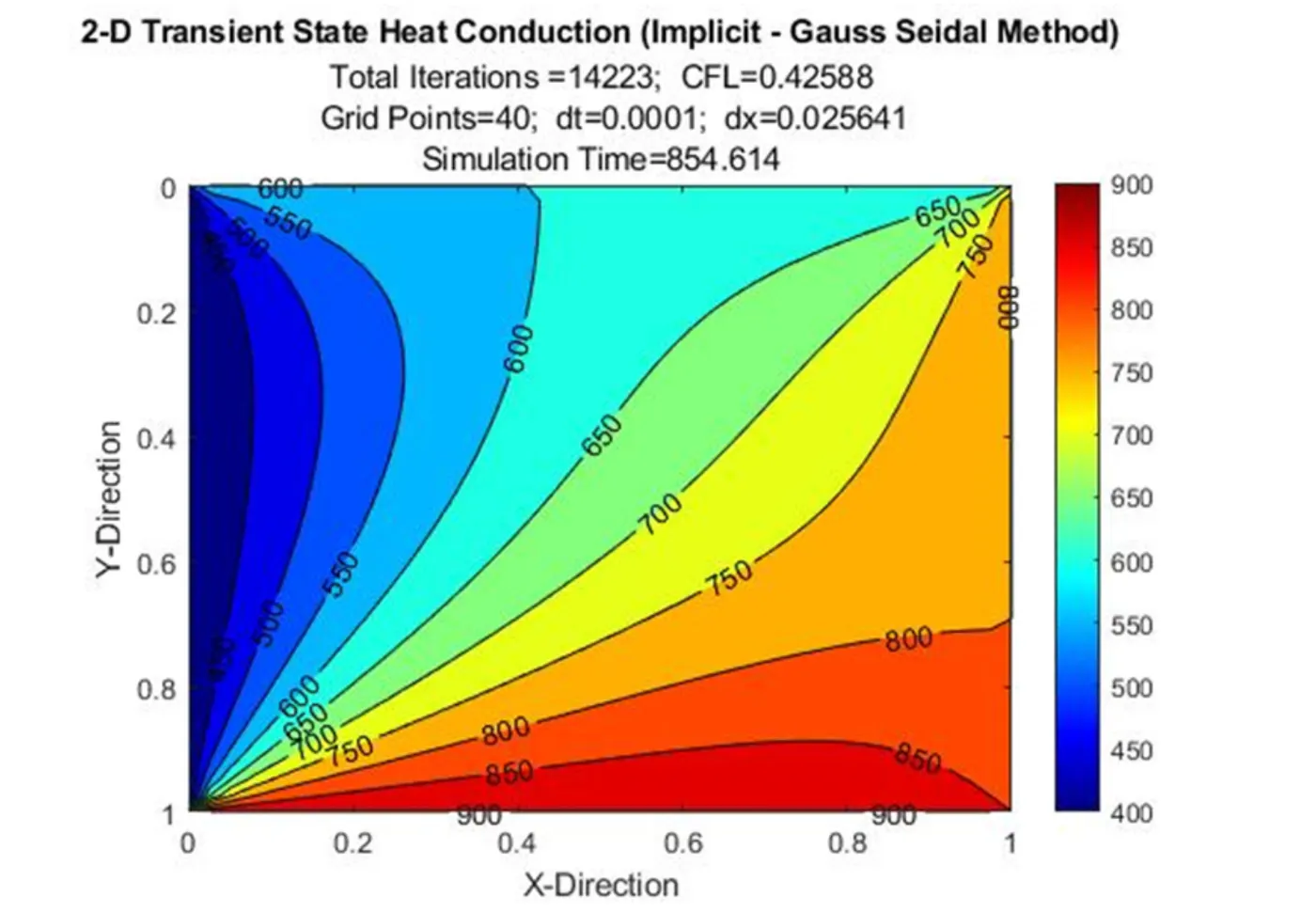
1.The plot implicitly represents the temperature distribution along the x and y axes for the transient state analysis of the 2-D heat conduction equation.
2.By graphing the temperature at the domain's bottom, the greater temperature may be disseminated around the domain.
3.The Gauss Seidal Iterative technique is used for transient state analysis, and 14223 iterations are required to achieve steady-state convergence for the domain.
4.The convergence loop is executed within the time loop "nt," where the older temperature value and prior time step temperature values are updated correspondingly.
The Gauss Seidal technique converges quicker than the Jacobi Iterative approach.

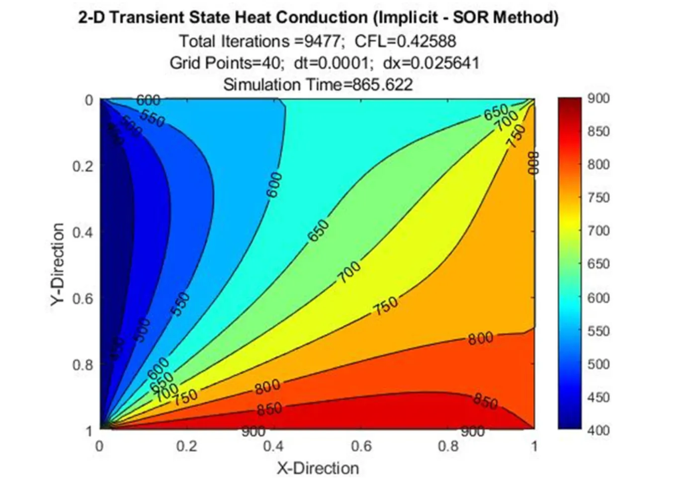
1.The plot implicitly represents the temperature distribution along the x and y axes for the transient state analysis of the 2-D heat conduction equation.
2.By graphing the temperature at the domain's bottom, the greater temperature may be disseminated around the domain.
3.The Successive Over Relaxation Iterative approach is used for transient state analysis, and 9477 iterations are required to achieve steady-state convergence for the domain.
4.The convergence loop is executed within the time loop "nt," where the older temperature value and prior time step temperature values are updated correspondingly.
Based on the relaxation factor, the SOR Iterative approach converges quicker than the Jacobi Iterative method and the Gauss Seidal method.

Conclusion:

1.The numerical analysis of the 2D steady-state heat conduction equation is carried out through the application of iterative techniques, namely the Jacobi, Gauss-Seidel, and Successive Over Relaxation methods.

2.For the 2D transient heat conduction equation, numerical analysis is performed using both Explicit and Implicit methods. The thermal diffusivity value, denoted by α=1.4, is chosen to facilitate the diffusion of temperature distribution during transient heat conduction.

3.The relaxation factor ω is set to 1.2. In the SOR method, if the relaxation factor exceeds this value, the iterations tend to exceed the target value, leading to prolonged computation time compared to the Gauss-Seidel method.

4.Both the transient and steady-state analyses of the 2D heat conduction equation are conducted, revealing the temperature distribution across the domain in accordance with the defined boundary conditions.

5.In the context of the steady-state analysis, the SOR iterative method achieves faster convergence compared to the Gauss-Seidel and Jacobi methods.

6.In the case of the Explicit analysis in the transient state, the equations are directly solved within the time loop to obtain the desired temperature distribution along the x and y axes.

7.For the Implicit analysis in the transient state, a system of equations is solved using iterative techniques to achieve the convergence of steady-state solutions.

<!--[endif]--><!--[endif]-->