Week 9 - FVM Literature Review

Objectives:

The difference between FDM and FVM and to describe the need for interpolation schemes and flux limiters in Finite Volume Method (FVM).

Introduction:

There are 3 numerical method based solvers to solve the governing equations they are:

1.Finite Element Method (FEM)

2. Finite Difference Method (FDM)

3. Finite Volume Method (FVM)

Efficient techniques for CFD using the finite-difference and finite-volume methods has grown in popularity and has been used for a long time.

Finite Element Method (FEM)

The Finite Element Method (FEM) is a numerical approach for solving partial differential equations and variational problems by splitting the computational domain into smaller, simpler geometric forms known as elements. FEM is widely used in engineering and physics to analyse and simulate physical processes such as structural mechanics, heat transfer, fluid dynamics, and electromagnetics.

Finite Difference Method (FDM)

To limit the computational domain, boundary conditions are required. They symbolise communication with the outside world, which we do not wish to incorporate in our simulation. We may easily run into challenges managing borders for the purpose of determining the boundary conditions when using the finite-difference approach.

The finite-difference technique is the most simple method for discretizing a PDE based on its differential form. Consider a location in space where the continuum representation of the equations is replaced by a set of discrete equations known as finite-difference equations.

The finite-difference approach is commonly specified on a regular/structured grid (that is, the computational domain is typically split into hexahedral cells (the grid), and the solution is achieved at each nodal point). This knowledge may be leveraged to create extremely efficient solution approaches. Regular grids are useful for supercomputer simulations at very large scales. The method is therefore not usually used for irregular CAD geometries, but more often for rectangular or block-shaped models.

For example, the Formula One car computational-fluid-dynamic (CFD) simulations and space-shuttle CFD simulations. When dealing with material discontinuities, the finite-difference approach is more difficult to employ. Furthermore, it is unsuitable for local grid refinement or anything resembling "adaptive mesh refinement." This may be required to resolve local quick fluctuations in solutions, such as those discussed previously near a complicated shape's corner.

If the boundary-condition difficulty on curved boundaries is addressed, the approach produces highly efficient and high-quality results. Because the finite-difference approach is specified dimension by dimension, it is simple to increase the "element order" to achieve higher-order precision.

Finite Volume Method (FVM)

The finite-volume method, similar to the finite-difference method, divides the CAD model into extremely small yet finite-sized elements of geometrically basic forms. Aside from that, the finite-volume technique differs greatly from the finite-difference method, beginning with the idea of elements, which are now referred to as cells.

A discretization using the finite volume method (FVM) is based on an integral version of the PDE to be solved (e.g., conservation of mass, momentum, or energy) and can handle discontinuities in solutions. The PDE is formulated in a way that allows it to be solved for a given finite volume (or cell). The computing domain is discretized into finite volumes, and the governing equations are solved for each volume. The resultant system of equations frequently includes fluxes of the conserved variable, hence flux computation is critical in FVM.

The strength of the finite-volume technique is that it only requires flux assessment at the cell borders. This also applies to nonlinear issues, making it particularly effective for managing (nonlinear) conservation rules in transportation difficulties.

The finite-volume method's local precision, such as near to a point of interest, can be improved by improving the mesh surrounding that point. However, when utilising the finite-volume technique, the functions that approximate the solution cannot be easily created of higher order. When compared to the finite-difference approach, this is a drawback of the finite-volume method.

The primary benefit of this approach over FDM is that it does not need the usage of structured grids, and the work required to internally convert the provided mesh to a structured numerical grid is fully avoided. The resultant approximate solution is discrete, as with FDM, although the variables are often set at cell centres rather than nodal points. This is not always the case, as face-centred finite volume approaches exist. Interpolation is used to acquire the values of field variables in non-storage places (e.g., vertices).

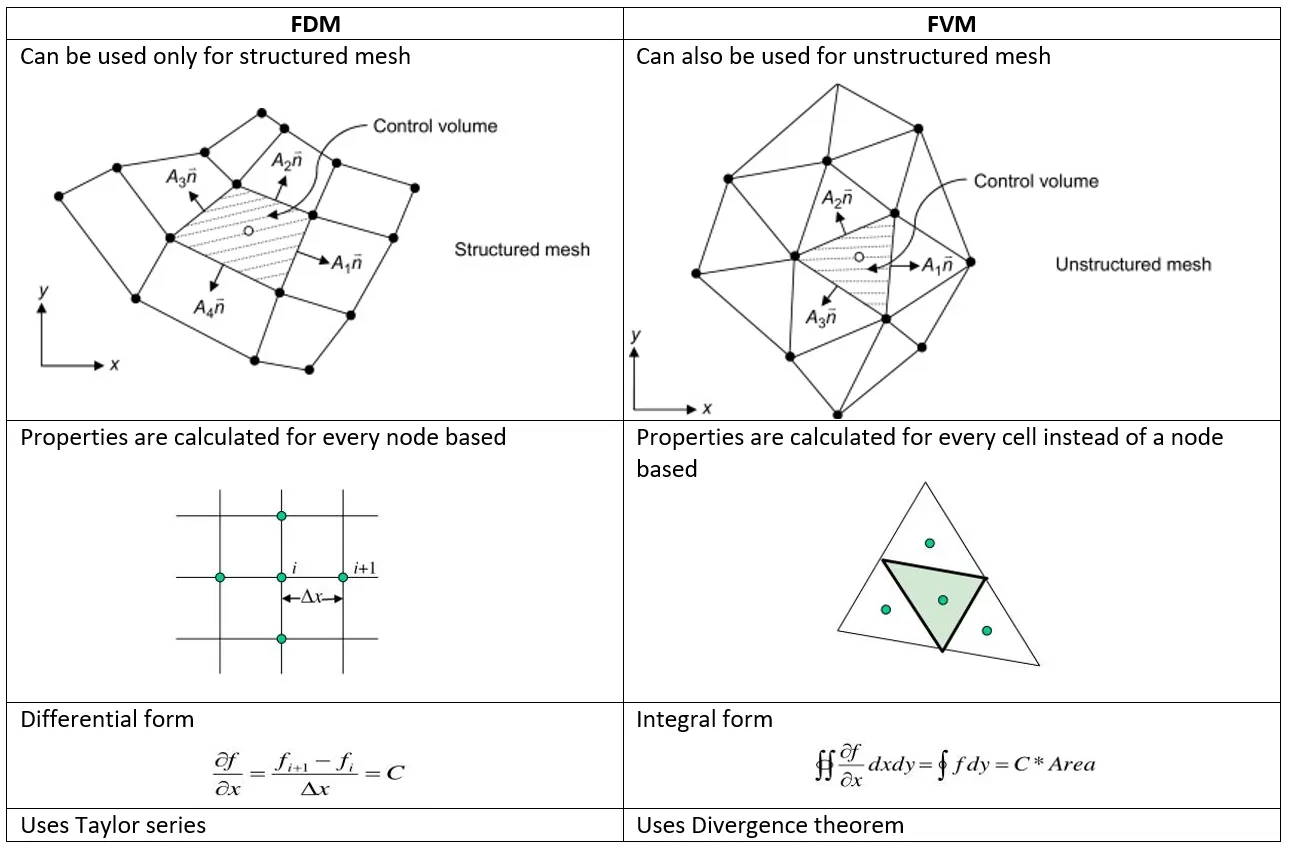
This table below shows some difference between the Finite Difference Method (FDM) and the Finite Volume Method (FVM)

Next let us see about the Interpolation Schemes:

INTERPOLATION SCHEMES:

Surface and volume integral approximations necessitate variable values at locations other than the control volume's computational nodes. Interpolation equations are used to acquire values at these locations.

Methods of interpolation:

1. Upwind interpolation

2. Linear interpolation

3. Quadratic upwind interpolation

4. Hybrid interpolation

UPWIND INTERPOLATION: (UDS)

Upwind interpolation is mostly utilised for convection-dominated issues. Depending on the flow direction, this interpolation approach is fundamentally comparable to utilising the forward difference method or the backward difference method. The variable value to be utilised in an interpolation process is determined by the direction of velocity at a specific place. We utilise the node upwind or upstream from the provided node, as the name implies.

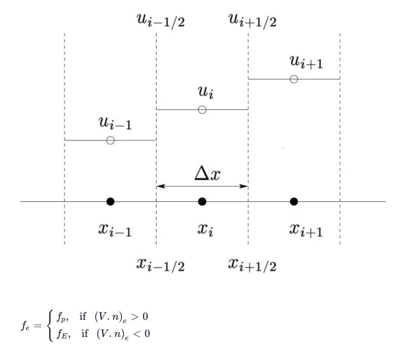
It is used in case of convection dominated problems. The upwind interpolation (UDS) for approximating the value of variable "fat the east face of the control volume is given by:

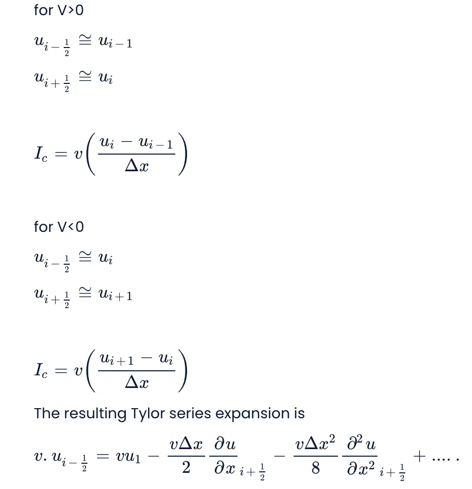
The values for the interface is given by

Upwind interpolation is the only approximation that unconditionally meets the boundedness criteria, in the sense that the solution will always stay bounded regardless of velocity values or grid spacing. This is an example of using upwind interpolation, which will never provide oscillatory solutions. The numerical diffusivity of upwind interpolation is high. If there are strong peaks or oscillatory values in the solution, they will be damped away due to the existence of numerical diffusion, and therefore numerical diffusion is exacerbated in multi-dimensional flows, Especially when the flow is oblique to the grid space. Peaks or fast fluctuations in the variables will be spread out as a result of the addition of an extra diffusive coefficient, known as a numerical diffusive coefficient when UDS is applied. Because it is first-order accurate, grids are necessary to achieve correct results.

Linear Interpolation(CDS):

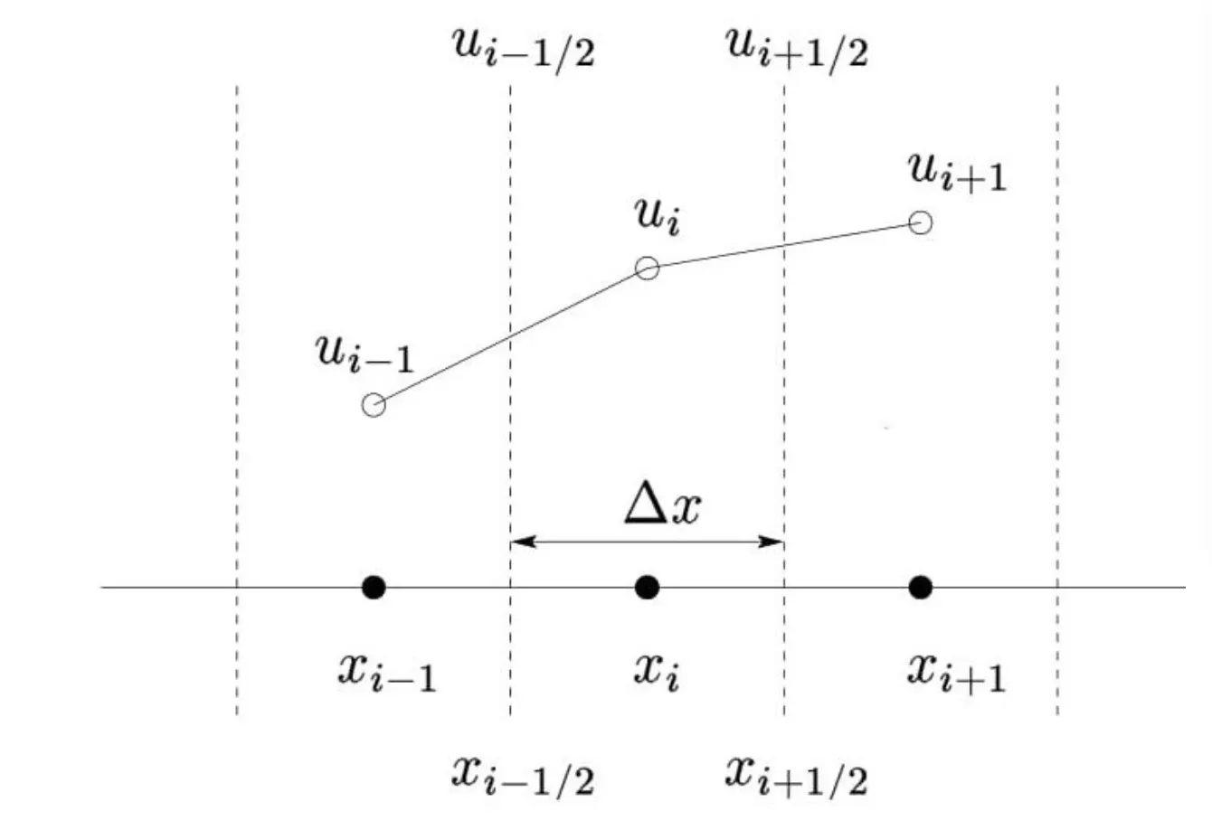
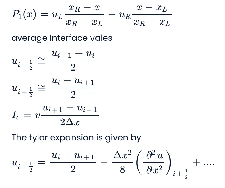
The approximated value of the variable at control volume centroid by linear interpolation of the values at two nearest computational nodes.

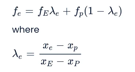
The linear interpolation is equivalent to the use of the CDS formula of the first-order derivative, and hence this scheme is also termed as Central Differencing Scheme(CDS). This is 2nd-order accurate and may produce oscillatory results therefore small grids are preferred for this method. This is one of the most widely used interpolation methods.

The linear interpolation is equalling to the use of central differencing formula of the first order derivative,

Interpolation Polynomial,

Quadratic Upwind Interpolation(QUICK):

QUICK, which stands for Quadratic Upstream Interpolation for Convective Kinematics, is a higher-order differencing system in computational fluid dynamics that uses a three-point upstream weighted quadratic interpolation for cell face values. There are several ways for solving the stable convection-diffusion equation in computational fluid dynamics. The central differencing scheme, upwind scheme, hybrid system, and QUICK scheme are some of the strategies employed.

A quadratic function travelling through two bracketing or surrounding nodes and one upstream node must be employed to get the cell face value. The first-order derivative is incorporated in the central differencing scheme and the second-order upwind scheme, whereas the second-order derivative is disregarded. As a result, these methods are deemed second-order accurate, whereas QUICK takes the second-order derivative into account but ignores the third-order derivative, making it third-order accurate. This system is used to solve convection-diffusion equations by employing second-order central difference for the diffusion term and first-order central difference for the convection term. It is third-order accurate in space and first-order correct in time. QUICK is best for steady or quasi-stationary strongly convective elliptic flow.

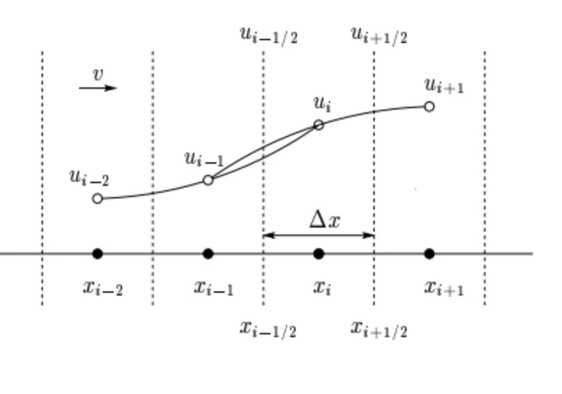
Interpolation Polynomial,

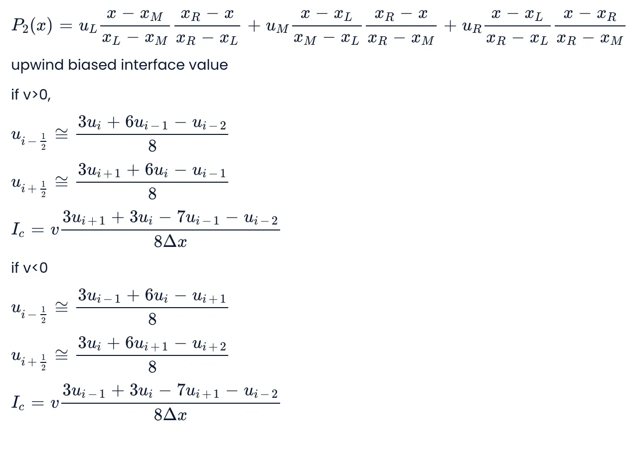
Hybrid Interpolation scheme:

This interpolation approach combines the central differencing scheme and the Upwind differencing scheme, both of which are based on the local pellet number. The following generic partial equation can describe it:

Here, ρ is density, 'u' is the velocity vector, T is the diffusion coefficient & Sf is the source term. In this equation property, f can be temperature, internal energy, or component of velocity vector u in x, y, and z directions.

For one-dimensional analysis of the convection-diffusion problem in steady-state and without the source, the equation reduces to,

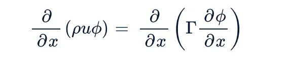
Where, 0 < x < L

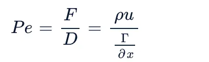
Peclet number (Pe) is a non-dimensional quantity used to measure the relative strengths of convection and diffusion, and it is denoted as:

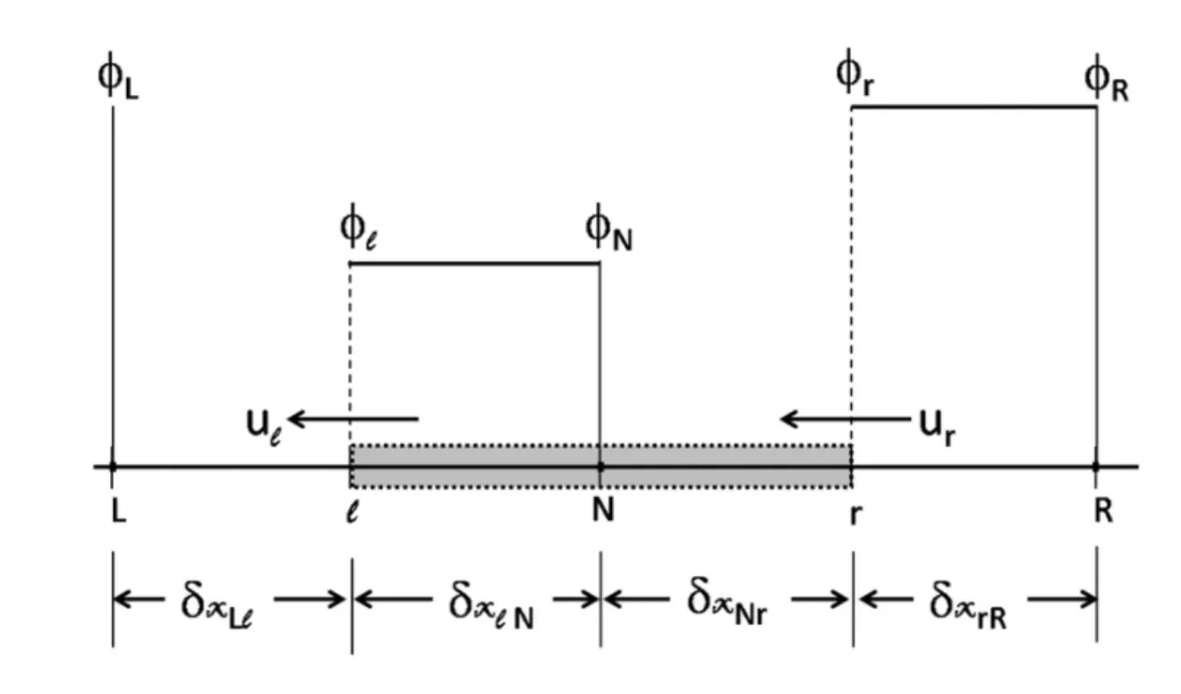
The grid used for discretization in Central Difference Scheme:

Flux Limiter:

A flux limiter, in the context of numerical methods for solving partial differential equations (PDEs), is a technique used to control the numerical diffusion or artificial dissipation in the solution. This is particularly important in high-resolution methods like finite volume or finite difference schemes, where the goal is to accurately capture sharp gradients or discontinuities in the solution.

The need for flux limiters arises when solving hyperbolic PDEs, such as those governing fluid dynamics or wave propagation. In these cases, traditional numerical methods can introduce spurious oscillations or smearing of sharp features in the solution. Flux limiters are employed to prevent these numerical artifacts and maintain the stability of the numerical solution.

The basic idea behind flux limiters is to modify the numerical fluxes across cell interfaces in a way that prevents unphysical overshoots or undershoots. This is often done by comparing the local gradients of the solution with a reference slope, and limiting the fluxes based on this information.

Flux Limiter functions are used to fine tune the higher order and lower order schemes in such a way that the resulting scheme gives a higher order accuracy in the smooth region of the flow and maintains first order accuracy in the vicinity of shocks and discontinuities. For such a scheme TVD scheme is employed.

F(ui+1/2)=f low(i+1/2)−ψ(ri)(flow(i+1/2)−f high(i+1/2))

F(ui−1/2)=f low(i−1/2)−ψ(ri−1)(flow(i−1/2)−f high(i−1/2))

where,

f low is low precision flux (first order)

f high is high precision flux (higher order)

Conclusion:

The Finite Volume Method (FVM) stands out as a robust and effective approach for solving Computational Fluid Dynamics (CFD) problems. By employing suitable interpolation schemes and implementing precise flux limiters, the Finite Volume Method enables the accurate resolution of a diverse array of CFD challenges.This numerical technique is particularly adept at handling complex fluid flow scenarios. The incorporation of interpolation schemes ensures the representation of fluid properties across the discretized computational domain, allowing for the accurate approximation of fluxes at cell interfaces.

One notable strength of the Finite Volume Method lies in its ability to address discontinuities within the flow field. Flux limiters play a crucial role in mitigating numerical artifacts that can arise, especially in the presence of sharp gradients or discontinuities. These limiters carefully control the transfer of information between adjacent computational cells, preventing spurious oscillations and maintaining the stability of the solution.