af(i)=af(i)</math>">af(i)=af(i)
bf(i+1)=bf(i)+bΔxf′(i)+bΔx22!f′′(i)+bΔx33!f′′′(i)+bΔx44!f′′′′(i)+bΔx55!f′′′′′(i)+bΔx66!f′′′′′′(i)+...</math>">bf(i+1)=bf(i)+bΔxf'(i)+(bΔx^2/2!)f''(i)+(bΔx^3/3!)f'''(i)+(bΔx^4/4!)f''''(i)+(bΔx^5/5!)f'''''(i)+(bΔx^6/6!)f''''''(i)+...
cf(i+2)=cf(i)+c(2Δx)f′(i)+c(2Δx)22!f′′(i)+c(2Δx)33!f′′′(i)+c(2Δx)44!f′′′′(i)+c(2Δx)55!f′′′′′(i)+c(2Δx)66!f′′′′′′(i)+...</math>">cf(i+2)=cf(i)+c(2Δx)f'(i)+(c(2Δx)^2/2!)f''(i)+(c(2Δx)^3/3!)f'''(i)+(c(2Δx)^4/4!)f''''(i)+(c(2Δx)^5/5!)f'''''(i)+(c(2Δx)^6/6!)f''''''(i)+...
df(i+3)=df(i)+d(3Δx)f′(i)+d(3Δx)22!f′′(i)+d(3Δx)33!f′′′(i)+d(3Δx)44!f′′′′(i)+d(3Δx)55!f′′′′′(i)+d(3Δx)66!f′′′′′′(i)+...</math>">df(i+3)=df(i)+d(3Δx)f'(i)+(d(3Δx)^2/2!)f''(i)+(d(3Δx)^3/3!)f'''(i)+(d(3Δx)^4/4!)f''''(i)+(d(3Δx)^5/5!)f'''''(i)+(d(3Δx)^6/6!)f''''''(i)+...
ef(i+4)=ef(i)+e(4Δx)f′(i)+e(4Δx)22!f′′(i)+e(4Δx)33!f′′′(i)+e(4Δx)44!f′′′′(i)+e(4Δx)55!f′′′′′(i)+e(4Δx)66!f′′′′′′(i)+...</math>">ef(i+4)=ef(i)+e(4Δx)f'(i)+(e(4Δx)^2/2!)f''(i)+(e(4Δx)^3/3!)f'''(i)+(e(4Δx)^4/4!)f''''(i)+(e(4Δx)^5/5!)f'''''(i)+(e(4Δx)^6/6!)f''''''(i)+...
gf(i+5)=gf(i)+g(5Δx)f′(i)+g(5Δx)22!f′′(i)+g(5Δx)33!f′′′(i)+g(5Δx)44!f′′′′(i)+g(5Δx)55!f′′′′′(i)+g(5Δx)66!f′′′′′′(i)+...</math>">gf(i+5)=gf(i)+g(5Δx)f'(i)+(g(5Δx)^2/2!)f''(i)+(g(5Δx)^3/3!)f'''(i)+(g(5Δx)^4/4!)f''''(i)+(g(5Δx)^5/5!)f'''''(i)+(g(5Δx)^6/6!)f''''''(i)+...
Adding the above equations we get
af(i)+bf(i+1)+cf(i+2)+df(i+3)+ef(i+4)+gf(i+5)=f(i)[a+b+c+d+e+g]+Δxf′(i)[b+2c+3d+4e+5g]+Δx2f′′(i)[b2+4c2+9d2+16e2+25g2]+Δx3f′′′(i)[b6+8c6+27d6+64e6+125g6]+Δx4f′′′′(i)[b24+16c24+81d24+256e24+625g24]+Δx5f′′′′′(i)[b120+32c120+243d120+1024e120+3125g120]</math>">af(i)+bf(i+1)+cf(i+2)+df(i+3)+ef(i+4)+gf(i+5)=f(i)[a+b+c+d+e+g]+Δxf'(i)[b+2c+3d+4e+5g]+Δx2f''(i)[b2+4c2+9d2+16e2+25g2]+Δx3f'''(i)[b6+8c6+27d6+64e6+125g6]+Δx4f''''(i)[b24+16c24+81d24+256e24+625g24]+Δx5f'''''(i)[b120+32c120+243d120+1024e120+3125g120]
In the above equations, we want only the coefficients of Δx2f′′(i)</math>">Δx2f''(i) and we assume the coefficient to be one and for the remaining terms we assume the coefficients to be zero.
a+b+c+d+e+g=0</math>">a+b+c+d+e+g=0
b+2c+3d+4e+5g=0</math>">b+2c+3d+4e+5g=0
b2+4c2+9d2+16e2+25g2=1</math>">b/2+4c/2+9d/2+16e/2+25g/2=1
b6+8c6+27d6+64e6+125g6=0</math>">b/6+8c/6+27d/6+64e/6+125g/6=0
b24+16c24+81d24+256e24+625g24=0</math>">b/24+16c/24+81d/24+256e/24+625g/24=0
b120+32c120+243d120+1024e120+3125g120=0</math>">b/120+32c/120+243d/120+1024e/120+3125g/120=0
| Taylor Table |
| Assumed Function |
Taylor Series Expansion |
| f(i)</math>">f(i) |
Δf′(i)</math>">Δf'(i) |
Δx2f′′(i)</math>">Δx2f''(i) |
Δx3f′′′(i)</math>">Δx3f'''(i) |
Δx4f′′′′(i)</math>">Δx4f''''(i) |
Δx5f′′′′′(i)</math>">Δx5f'''''(i) |
Δx6f′′′′′′(i)</math>">Δx6f''''''(i) |
| |
af(i)</math>">af(i) |
a</math>">a |
0</math>">0 |
0</math>">0 |
0</math>">0 |
0</math>">0 |
0</math>">0 |
0</math>">0 |
| bf(i+1)</math>">bf(i+1) |
b</math>">b |
b</math>">b |
b2</math>">b/2 |
b6</math>">b/6 |
b24</math>">b/24 |
b120</math>">b/120 |
b720</math>">b/720 |
| cf(i+2)</math>">cf(i+2) |
c</math>">c |
2c</math>">2c |
4c2</math>">4c/2 |
8c6</math>">8c6 |
16c24</math>">16c/24 |
32c120</math>">32c/120 |
64c720</math>">64c/720 |
| df(i+3)</math>">df(i+3) |
d</math>">d |
3d</math>">3d |
9d2</math>">9d/2 |
27d6</math>">27d/6 |
81d24</math>">81d/24 |
243d120</math>">243d/120 |
729d720</math>">729d/720 |
| ef(i+4)</math>">ef(i+4) |
e</math>">e |
4e</math>">4e |
16e2</math>">16e/2 |
64e6</math>">64e/6 |
256e24</math>">256e/24 |
1024e120</math>">1024e/120 |
(4096e)720</math>">4096e/720 |
| gf(i+5)</math>">gf(i+5) |
g</math>">g |
5g</math>">5g |
25g2</math>">25g/2 |
125g6</math>">125g/6 |
625g24</math>">625g/24 |
3125g120</math>">3125g/120 |
15625g720</math>">15625g/720 |
| Sum of Coefficients |
0 |
0 |
1 |
0 |
0 |
0 |
0 |
The Matlab code,
>> A=[1 1 1 1 1 1;0 1 2 3 4 5;0 1/2 4/2 9/2 16/2 25/2;0 1/6 8/6 27/6 64/6 125/6;0 1/24 16/24 81/24 256/24 625/24;0 1/120 32/120 243/120 1024/120 3125/120]
B=[0;0;1;0;0;0]
X=AB
A =
1.0000 1.0000 1.0000 1.0000 1.0000 1.0000
0 1.0000 2.0000 3.0000 4.0000 5.0000
0 0.5000 2.0000 4.5000 8.0000 12.5000
0 0.1667 1.3333 4.5000 10.6667 20.8333
0 0.0417 0.6667 3.3750 10.6667 26.0417
0 0.0083 0.2667 2.0250 8.5333 26.0417
B =
0
0
1
0
0
0
X =
3.7500
-12.8333
17.8333
-13.0000
5.0833
-0.8333
The equation using the Taylors Table is,
∂2y∂x2=af(i)+bf(i+1)+cf(i+2)+df(i+3)+ef(i+4)+gf(i+5)Δx2</math>">∂^2y/∂x^2=af(i)+bf(i+1)+cf(i+2)+df(i+3)+ef(i+4)+gf(i+5)/Δx^2
3) skewed left-sided difference
The equation may be used to calculate the number of Nodes necessary for 4th order approximation of a second-order derivative.
N=P+Qwhere
N denotes the number of nodes.
Q is the derivative order.
P is the approximation order.
So, in order to calculate the 2nd order derivative with the 4th order of approximation, we need 6 nodes.
the value of ∂2y∂x2</math>">∂^2y/∂x^2 with the 4th order of approximation is given by the equation
∂2y∂x2=af(i)+bf(i-1)+cf(i-2)+df(i-3)+ef(i-4)+gf(i-5)</math>">∂^2y/∂x^2=af(i)+bf(i−1)+cf(i−2)+df(i−3)+ef(i−4)+gf(i−5)
Taylor Table
| Assumed Function |
Taylor Series Expansion |
| f(i)</math>">f(i) |
Δxf′(i)</math>">Δxf'(i) |
Δx2f′′(i)</math>">Δx2f''(i) |
Δx3f′′′(i)</math>">Δx3f'''(i) |
Δx4f′′′′(i)</math>">Δx4f''''(i) |
Δx5f′′′′′(i)</math>">Δx5f'''''(i) |
Δx6f′′′′′′(i)</math>">Δx6f''''''(i) |
| |
af(i)</math>">af(i) |
a</math>">a |
0</math>">00 |
0</math>">0 |
0</math>">0 |
0</math>">0 |
0</math>">0 |
0</math>">0 |
| bf(i-1)</math>">bf(i−1) |
b</math>">b |
-b</math>">−b |
b2</math>">b/2 |
-b6</math>">−b/6 |
b24</math>">b/24 |
-b120</math>">−b/120 |
b720</math>">b/720 |
| cf(i-2)</math>">cf(i−2) |
c</math>">c |
-2c</math>">−2c |
4c2</math>">4c/2 |
-8c6</math>">−8c/6 |
16c24</math>">16c/24 |
-32c120</math>">−32c/120 |
64c720</math>">64c/720 |
| df(i-3)</math>">df(i−3) |
d</math>">d |
-3d</math>">−3d |
9d2</math>">9d/2 |
-27d6</math>">−27d/6 |
81d24</math>">81d/24 |
-243d120</math>">−243d/120 |
729d720</math>">729d/720 |
| ef(i-4)</math>">ef(i−4) |
e</math>">e |
-4e</math>">−4e |
16e2</math>">16e/2 |
-64e6</math>">−64e/6 |
256e24</math>">256e/24 |
-1024e120</math>">−1024e/120 |
(4096e)720</math>">4096e/720 |
| gf(i-5)</math>">gf(i−5) |
g</math>">g |
-5g</math>">−5g |
25g2</math>">25g/2 |
-125g6</math>">−125g/6 |
625g24</math>">625g/24 |
-3125g120</math>">−3125g/120 |
15625g720</math>">15625g/720 |
| Sum of Coefficients |
0 |
0 |
1 |
0 |
0 |
0 |
0 |
The Matlab code,
>> A=[1 1 1 1 1 1;0 -1 -2 -3 -4 -5;0 1/2 4/2 9/2 16/2 25/2;0 -1/6 -8/6 -27/6 -64/6 -125/6;0 1/24 16/24 81/24 256/24 625/24;0 -1/120 -32/120 -243/120 -1024/120 -3125/120]
B=[0;0;1;0;0;0]
X=AB
A =
1.0000 1.0000 1.0000 1.0000 1.0000 1.0000
0 -1.0000 -2.0000 -3.0000 -4.0000 -5.0000
0 0.5000 2.0000 4.5000 8.0000 12.5000
0 -0.1667 -1.3333 -4.5000 -10.6667 -20.8333
0 0.0417 0.6667 3.3750 10.6667 26.0417
0 -0.0083 -0.2667 -2.0250 -8.5333 -26.0417
B =
0
0
1
0
0
0
X =
3.7500
-12.8333
17.8333
-13.0000
5.0833
The equation using the Taylors Table is,
∂2y∂x2=af(i)+bf(i-1)+cf(i-2)+df(i-3)+ef(i-4)+gf(i-5)Δx2</math>">∂^2y/∂x^2=af(i)+bf(i−1)+cf(i−2)+df(i−3)+ef(i−4)+gf(i−5)
∂2y∂x2=af(i)+bf(i-1)+cf(i-2)+df(i-3)+ef(i-4)+gf(i-5)Δx2</math>">Main code:
clear
close
clc
%analytical fucntion=(e^x)cos(x);
%analytical derivative
%f(x)=(e^x)cos(x)
%f'(x)=(e^x)cos(x)-(e^x)sin(x)=e^x[cosx-sinx]
%f''(x)=(e^x)cos(x)-(e^x)sin(x)-[(e^x)sin(x)+(e^x)cos(x)]
%f''(x)=-2*e^x*sin(x)
%given inputs
x=pi/3; �rivative to be computed at x=pi/3
dx=linspace(pi/4000,1.5*pi,2000); %grid spacing dx=(pi*(4000-1.5))/(4000*2000)
%analytical derivative
analytical_derivative=-2*exp(x)*sin(x);
%creating Anonymous Function
f=@(x) exp(x)*cos(x);
%Skewed right-sided(4th order approimation)
%Solving for the coefficients
A=[1 1 1 1 1 1;0 1 2 3 4 5;0 1/2 4/2 9/2 16/2 25/2;0 1/6 8/6 27/6 64/6 125/6;0 1/24 16/24 81/24 256/24 625/24;0 1/120 32/120 243/120 1024/120 3125/120];
B=[0;0;1;0;0;0];
x_r=A*B;
%Skewed left-sided(4th order approimation)
%Solving for the coefficients
C=[1 1 1 1 1 1;0 -1 -2 -3 -4 -5;0 1/2 4/2 9/2 16/2 25/2;0 -1/6 -8/6 -27/6 -64/6 -125/6;0 1/24 16/24 81/24 256/24 625/24;0 -1/120 -32/120 -243/120 -1024/120 -3125/120];
D=[0;0;1;0;0;0];
x_l=C*D;
�ntral differencing(4th order approimation)
%Solving for the coefficients
E=[1, 1, 1, 1, 1;-2, -1, 0, 1, 2;4/2, 1/2, 0, 1/2, 4/2;-8/6, -1/6, 0, 1/6, 8/6;16/24, 1/24, 0, 1/24, 16/24];
F=[0;0;1;0;0];
x_c=E*F;
for i=1:length(dx)
%numerical derivative
%Skewed right-sided(4th order approimation)
%f''(x)=af(i)+bf(i+1)+cf(i+2)+df(i+3)+ef(i+4)+gf(i+5)
nd_right_difference(i)= (x_r(1)*f(x)+x_r(2)*f(x+dx(i))+x_r(3)*f(x+2*dx(i))+x_r(4)*f(x+3*dx(i))+x_r(5)*f(x+4*dx(i))+x_r(6)*f(x+5*dx(i)))/(dx(i)^2);
%Skewed left-sided(4th order approimation)
%f''(x)=af(i)+bf(i-1)+cf(i-2)+df(i-3)+ef(i-4)+gf(i-5)
nd_left_difference(i)=(x_l(1)*f(x)+x_l(2)*f(x-dx(i))+x_l(3)*f(x-2*dx(i))+x_l(4)*f(x-3*dx(i))+x_l(5)*f(x-4*dx(i))+x_l(6)*f(x-5*dx(i)))/(dx(i)^2);
�ntral differencing(4th order approimation)
%f''(x)=af(i-2)+bf(i-1)+cf(i)+df(i+1)+ef(i+2)
nd_cent_difference(i)=(x_c(1)*f(x-2*dx(i))+x_c(2)*f(x-1*dx(i))+x_c(3)*f(x)+x_c(4)*f(x+dx(i))+x_c(5)*f(x+2*dx(i)))/(dx(i)^2);
�solute error at x = pi/3
error_r(i)=abs(analytical_derivative-nd_right_difference(i));
error_l(i)=abs(analytical_derivative-nd_left_difference(i));
error_c(i)=abs(analytical_derivative-nd_cent_difference(i));
error=[error_r;error_l;error_c];
end
%Plotting the Absolute Error Curves
figure(1)
loglog(dx,error_r) %Plot both the axis on the log scale
grid on
hold on
loglog(dx,error_l)
loglog(dx,error_c)
ylabel('Absolute Error (Log Scale)')
xlabel('Grid Spacing (dx in Log Scale)')
legend('Right Differencing','Left Differencing','Central Differencing')
title('Absolute Error Comparison')
Result:
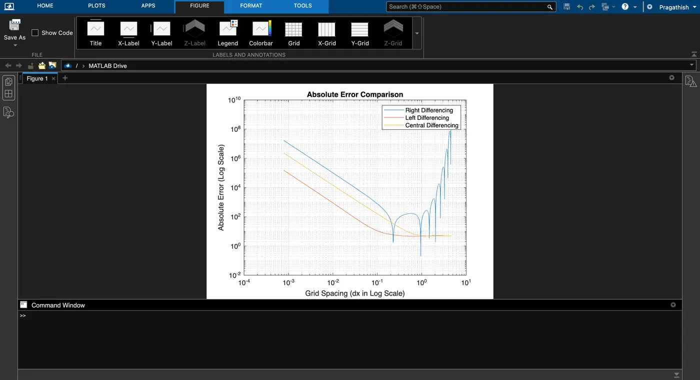
The graph above compares the absolute error for the left, right, and centre differencing schemes. The graph demonstrates that the centre scheme is more accurate than the skewed differencing. The curves also illustrate that the approximation function becomes unstable when the value of dx is very small or very big. This instability is generated by the interaction of many errors, including roundoff error, residual error, and truncation error.