Week 10 - Simulating Combustion of Natural Gas.

Aim: To Perform Combustion analysis of the Natural gas on a given combustor model.

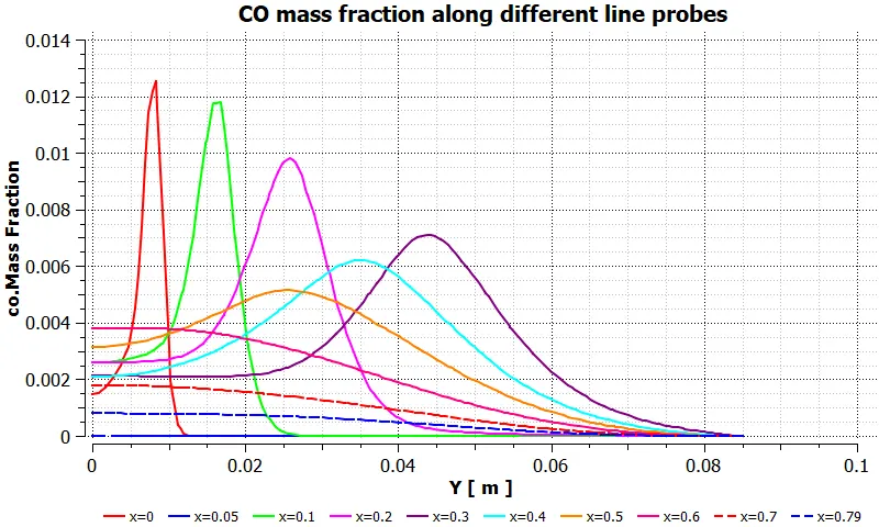
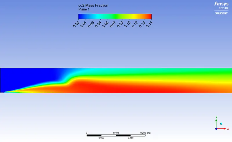
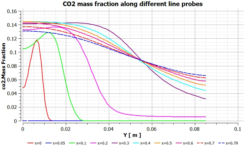
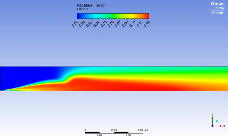
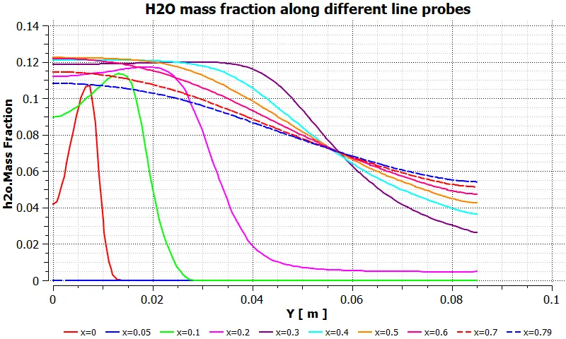
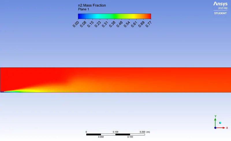
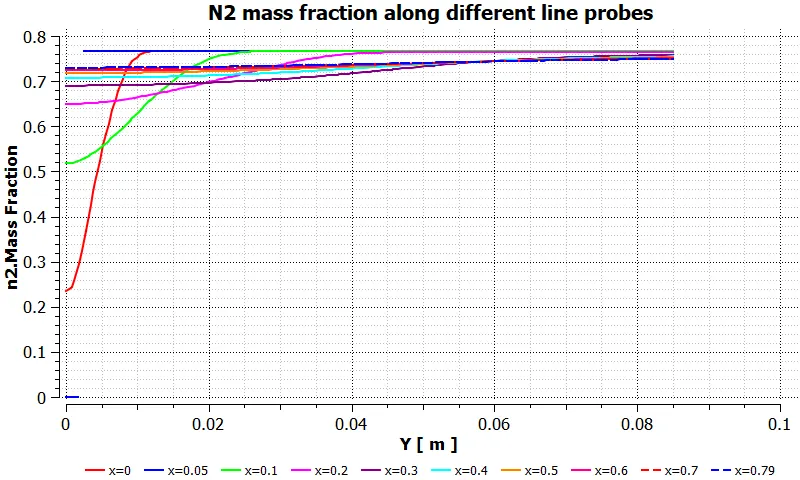
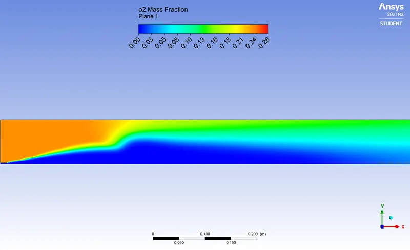
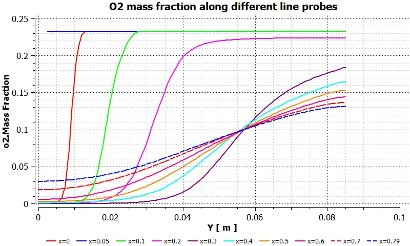
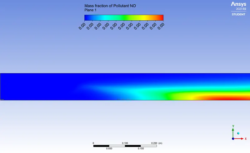
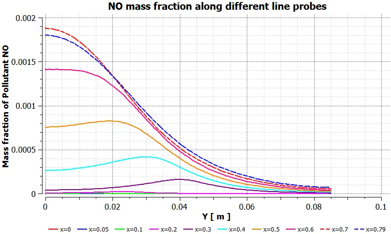
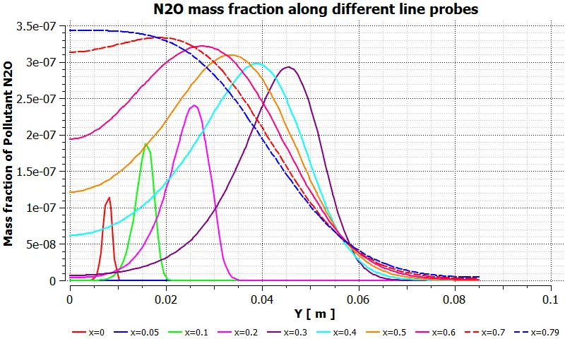
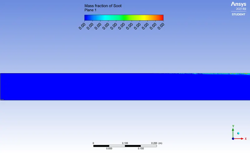
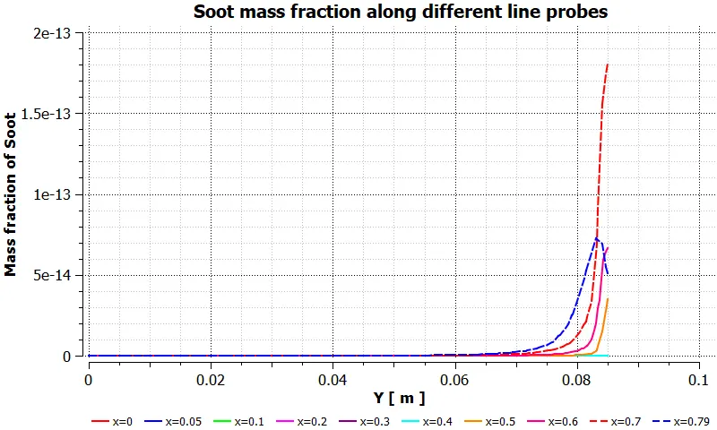
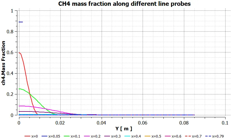
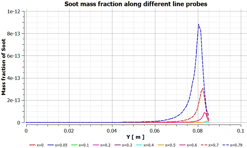
1. To Perform a combustion simulation on the combustor model and plot the variation of the mass fraction of the different species in the simulation using line probes at different locations of the combustor. Plot for species CO2, H2O, CH4, N2, O2, NOx emissions & Soot formation.

2. To check the effect of adding the water in the fuel. Vary the water content in the fuel from 5% to 30% by mole and observe the effect of it on the results by using the parametric study approach.

Theory:

Combustion:

Combustion is defined as the chemical reaction in which the fuel, mainly hydrocarbons, reacts with the oxidants and liberates energy in the form of heat.

In general combustion is a very complex phenomenon as this chemical reaction has various intermediary unstable steps which result in the release of heat and other forms of energy but heat is the major part of total energy released.

Combustion of Natural gas:
The general reaction of combustion of natural gas is represented as `CH_4 + a_r (O_2 + 3.76 N_2) => aCO_2 + bH_2 O + cN_2` .

After balancing out the above chemical reaction we get
`a = 1`;
`b = 2`;
`a_r = 2`; & `c = 7.52` .

Thus ,
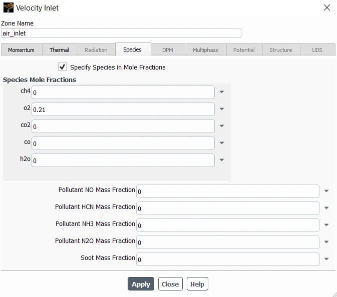
1) mole fraction of `O_2` in the supplied air = `frac{2 "moles of" O_2}{2 "moles of" O_2 + 7.52 "moles of" N_2}` =`frac{2}{9.52}`=0.21

2) mole fraction of `N_2` in the supplied air = `frac{7.52 "moles of" N_2}{2 "moles of" O_2 + 7.52 "moles of" N_2}` =`frac{7.52}{9.52}`=0.79

Similarly

1) mass fraction of `O_2` in the supplied air = `frac{2 "moles of" O_2 xx 16}{(2 "moles of" O_2 xx 16) + (7.52 "moles of" N_2 xx 14)}` =`frac{32}{137.28}`=0.23

2) mole fraction of `N_2` in the supplied air = `frac{7.52 "moles of" N_2 xx 14}{(2 "moles of" O_2 xx 16) + (7.52 "moles of" N_2 xx 14)}` =`frac{105.28}{137.28}`=0.79

Types of Combustion Simulation:
The simulation of combustion can be divided into two types-

• Combustion based on Mixing
  • Non-Premixed Combustion:
    In non-premixed combustion, fuel and oxidizer enter the reaction zone in distinct streams.
    It occurs during direct injection or late injection of fuel in IC engines.
    Examples of non-premixed combustion includes pulverised coal furnaces, diesel internal-combustion engines and pool fires.
  • Premixed Combustion:
    In premixed combustion,fuel and oxidizer are mixed at the molecular level prior to ignition.
    Combustion occurs as flames front propagate into the unburnt reactants.
    Examples of premixed combustion is the carburetor fixed upstream of the engine.
  • Partially Premixed Combustion:
    It lies in between the Non-premixed and Premixed Combustion.
    
    
• Combustion based on Phase
  • Fluid Phase (Volumetric Reactions)
    Combustion takes place in the fluid region.
  • Wall (Surface Reactions)
    Combustion takes place on the wall or a solid surface.
  • Particles ( Surface Reactions)
    Combustion takes place on the Lagrangian particles.
    Combustion of fine powdered coal is an example of particle combustion.
  • Porous Region
    Combustion takes place in a porous region.
    The reactions in an after-treatment system is the example of combustion in the porous regions.

In CFD modelling several combustion models are available are enlisted below

• Eddy dissipation model:
  The eddy dissipation model is based on the concept that chemical reaction is fast relative to the transport processes in the flow. When reactants mix at the molecular level, they instantaneously form products. The model assumes that the reaction rate may be related directly to the time required to mix reactants at the molecular level.The eddy dissipation model was developed for use in a wide range of turbulent reacting flows covering premixed and diffusion flames. Because of its simplicity and robust performance in predicting turbulent reacting flows, this model has been widely applied in the prediction of industrial flames.
  
  
• The finite chemistry model :
  The finite-rate chemistry model allows the computation of reaction rates described by the molecular interaction between the components in the fluid. It can be combined with the eddy dissipation model for flames where chemical reaction rates might be slow compared with the reactant mixing rates. The finite-rate chemistry model is best applied to situations where the chemical time scale is rate-limiting. This model can be used in conjunction with both laminar and turbulent flow.
  
  
• The Combination of Eddy dissipation model and Finite chemistry model is also used where the turbulent mixing time scale is calculated along with chemical reaction time scale and lower of the both is used for computations.

Part 1 - Workflow:

Geometry Preparation:

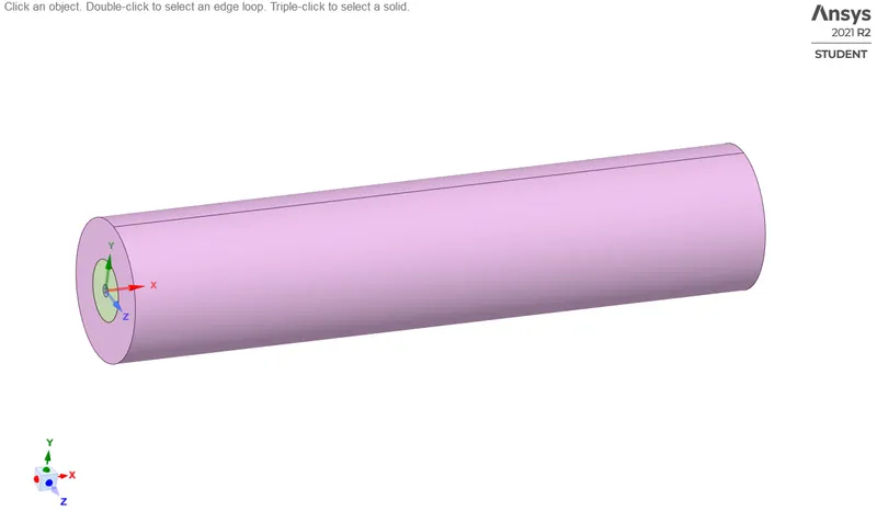
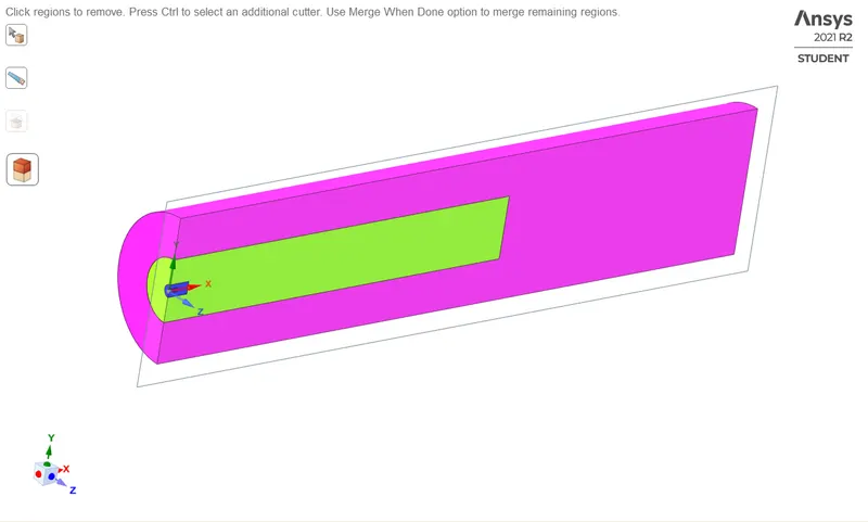
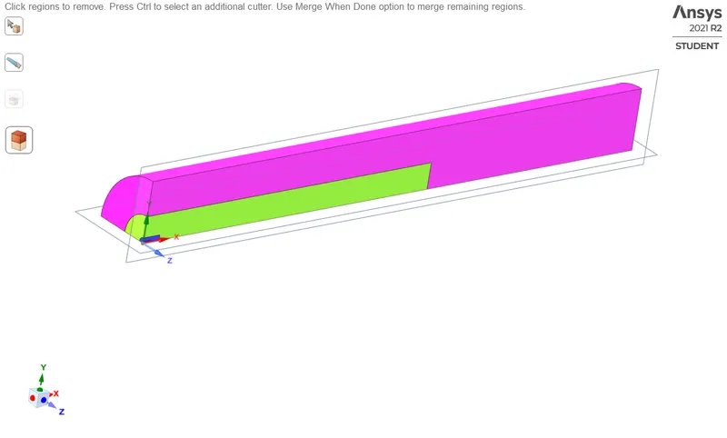
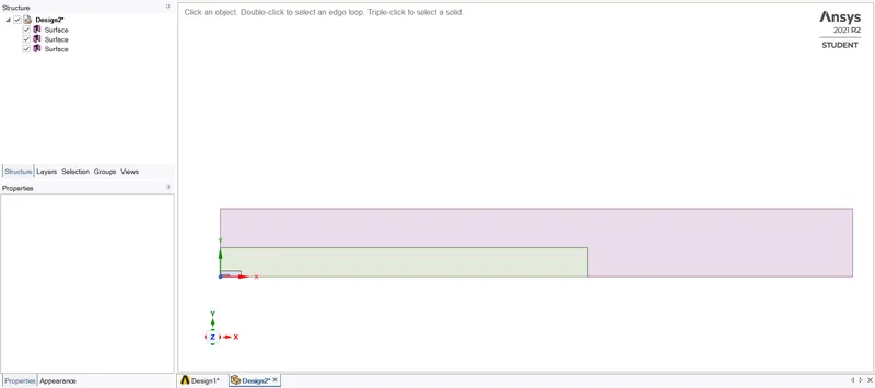
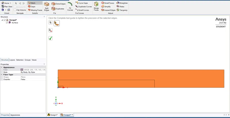
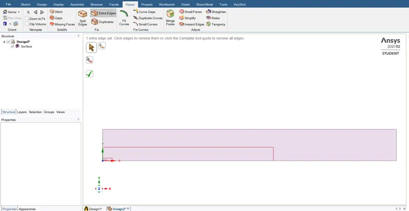
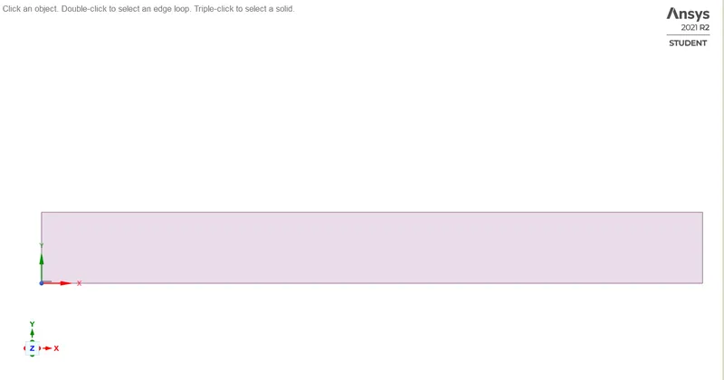
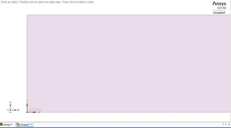
The 3D geometry model of the combustor has been given. As the combustor is cylindrical in design, the air and fuel enter the combustor longitudinally from one end. This makes the combustor geometry axis symmetric. Thus to minimise the computational time the required 2D geometry is obtained by using the split geometry utility, surface stitching utility and extra edge removal utility.

	3D Geometry -full			3D Split Geometry -half
	3D Split geometry - Quarter			2D Surface geometry by copying the surfaces
	Surface Stiching			Extra Edges removal
	Required 2D Geometry			Required 2D Geometry Magnified at inlet

Meshing:

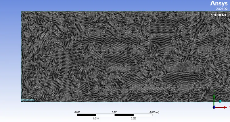
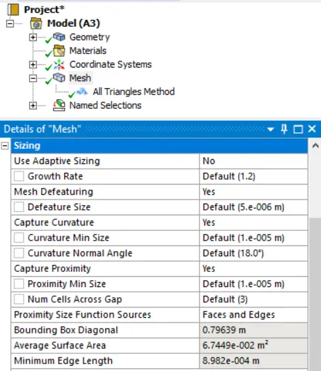
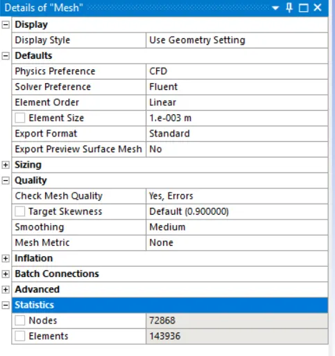
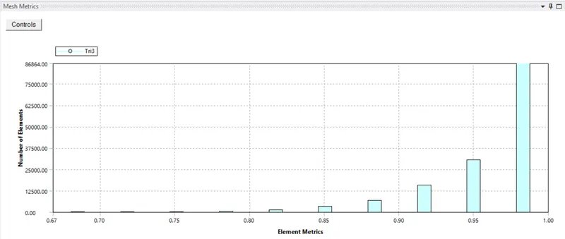
The geometry parts and boundaries have been named using named selection as air-inlet, fuel-inlet , outlet , axis and wall. The geometry is meshed with the all triangles method with the minimum size of 1 mm.

	Mesh			Mesh Method and Sizing details
	Mesh Details			MEsh Metrics

Case Setup:

Pressure based steady state solver with absolute velocity formation.

Axisymmetric 2D space setup selected. The x-axis is chosen as the axis of symmetry in the 2D geometry as the requirement of the Ansys Fluent.

Energy equations turned ON.

Viscous model: Standard k-epsilon turbulence model with standard wall functions.

Species: Species transport model has been selected. Along with that the Nox and Soot models are activated as follows

	Species transport Model settings		NOx model settings		Soot Model Settings

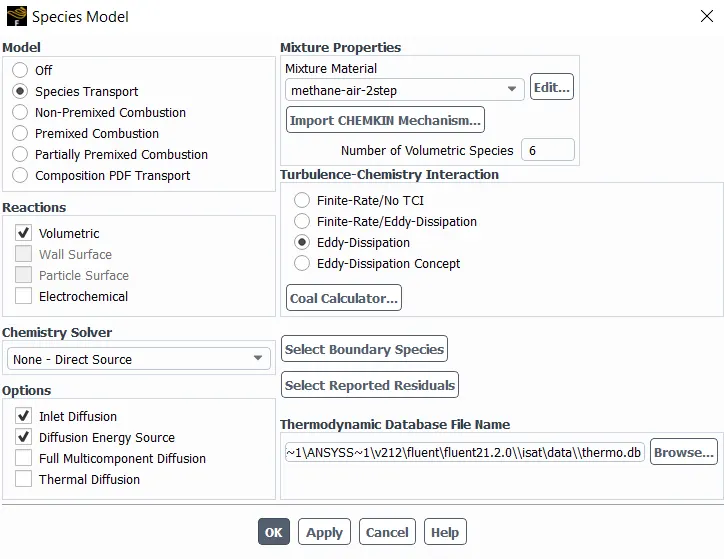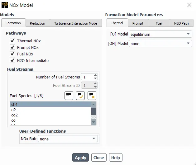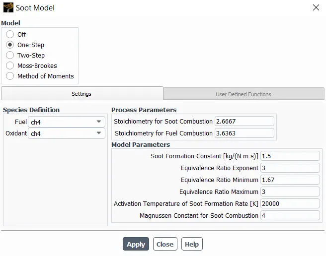Fluid zone condition: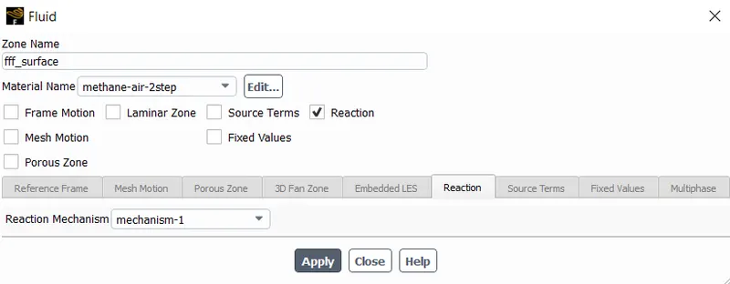

Boundary Conditions:

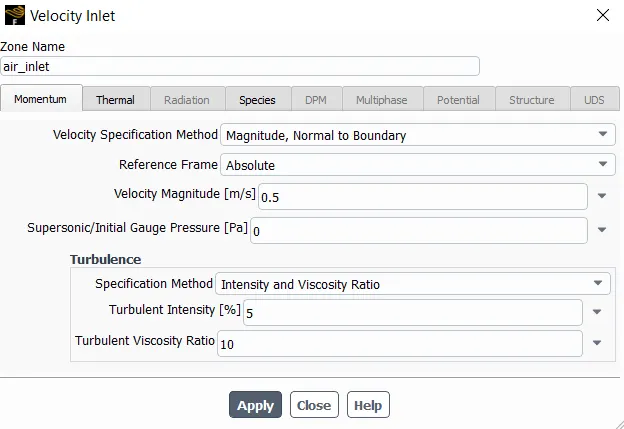
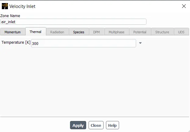
1) Air-inlet boundary conditions:

	Momentum settings		Thermal settings		Species Settings

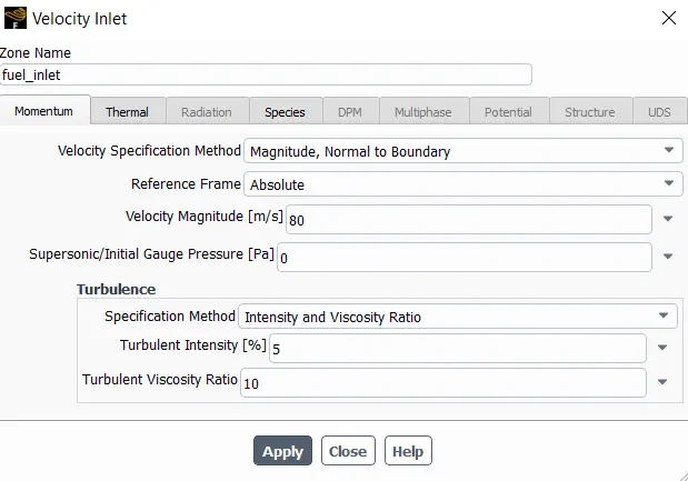
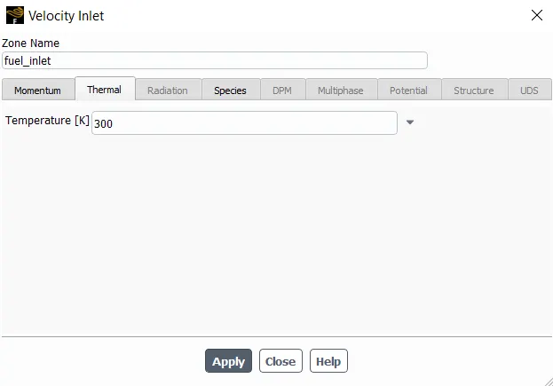
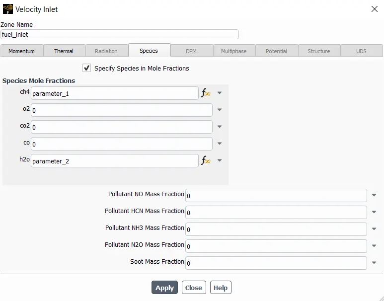
2) Fuel-inlet boundary conditions and input parameter settings:

	Momentum settings		Thermal settings		Species Settings

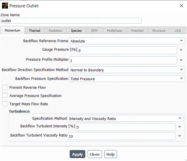
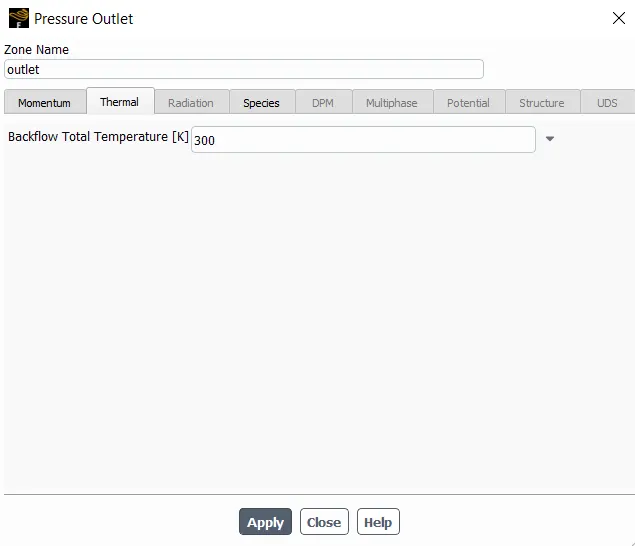
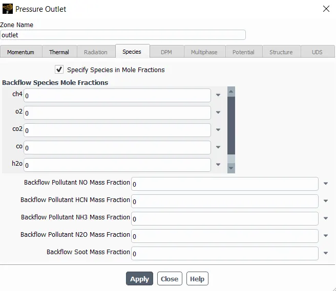
3) Outlet boundary conditions:

	Momentum settings		Thermal settings		Species Settings

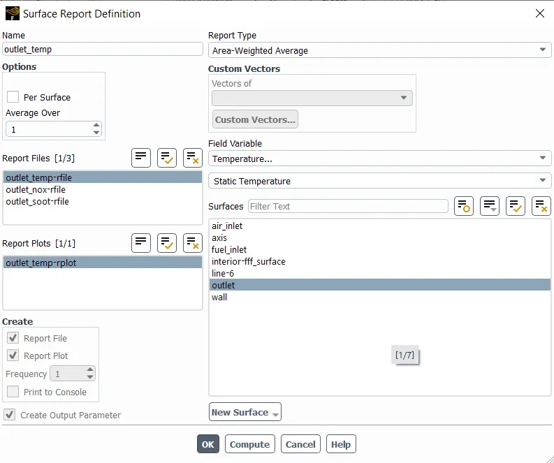
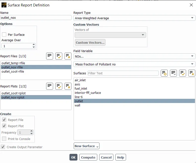
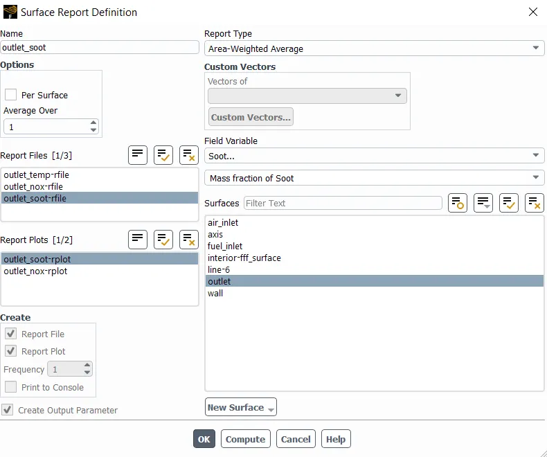
Report Definitions and Output parameter settings:

	Outlet Temperature		NOx at Outlet		Soot at Outlet

Solution Method and controls: SIMPLE scheme is selected for pressure velocity coupling.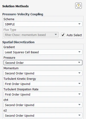

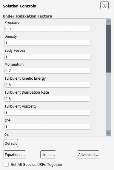
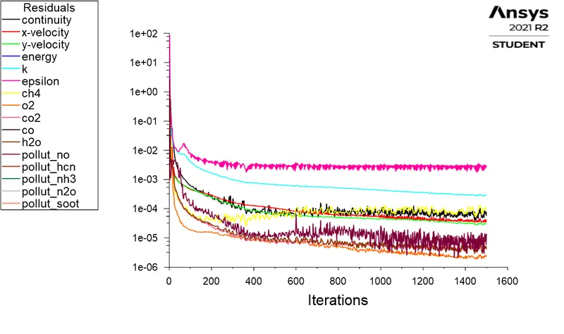
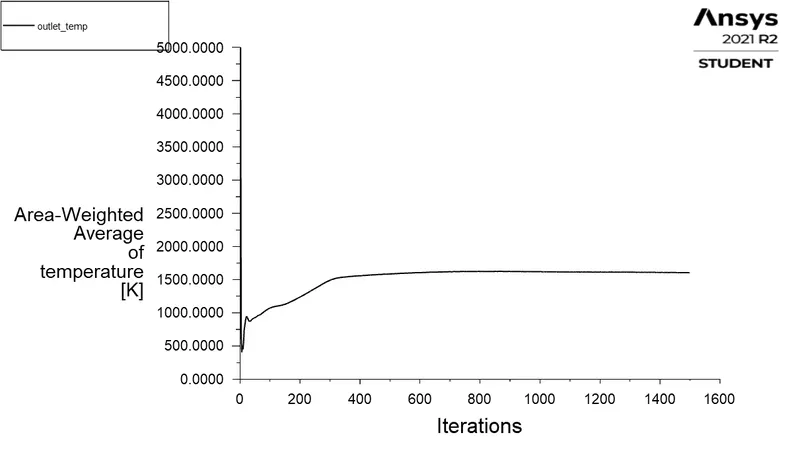
Initialisation and Reports: Hybrid initialisation is done and Simulation is done for 1500 number of iterations.

Post-Processing:
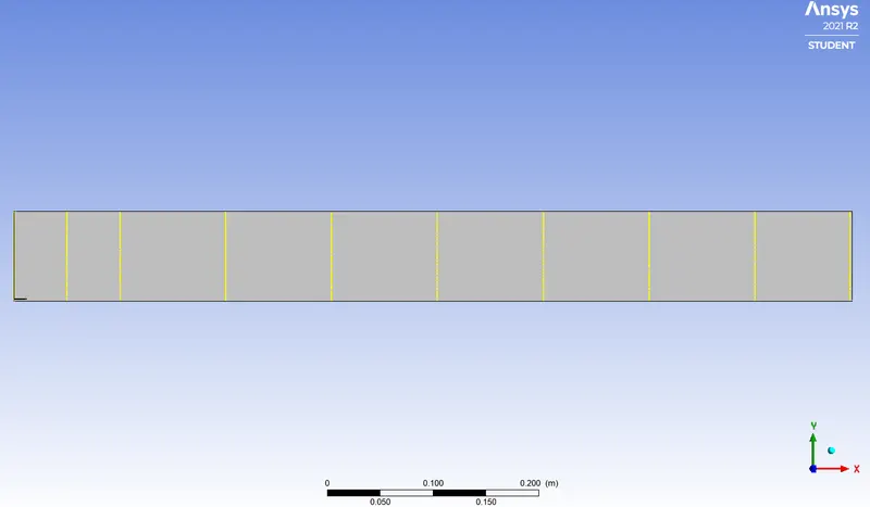
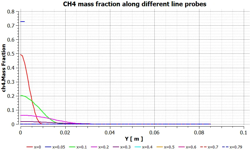
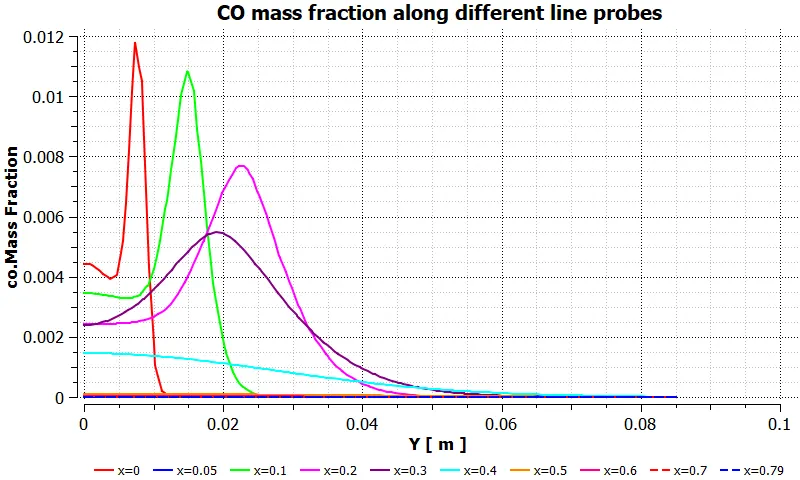
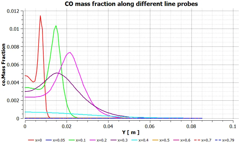
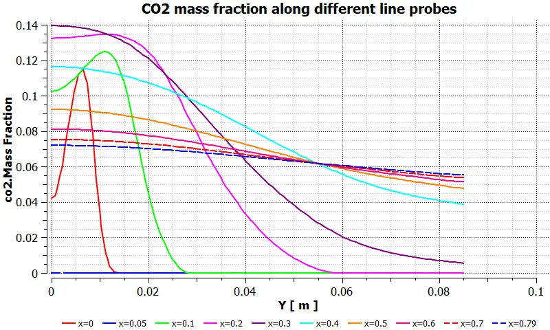
Line Probe settings:

1. Line 1 at x=0.0 m
2. Line 2 at x=0.05 m
3. Line 3 at x=0.1 m
4. Line 4 at x=0.2 m
5. Line 5 at x=0.3 m
6. Line 6 at x=0.4 m
7. Line 7 at x=0.5 m
8. Line 8 at x=0.6 m
9. Line 9 at x=0.7 m
10. Line 10 at x=0.79 m
    
    
    
    The require results are obtained and presented below

Results:

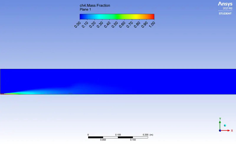
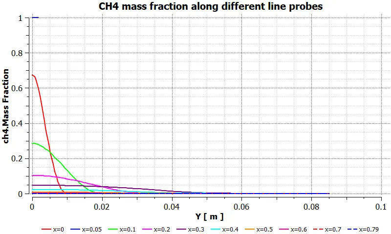
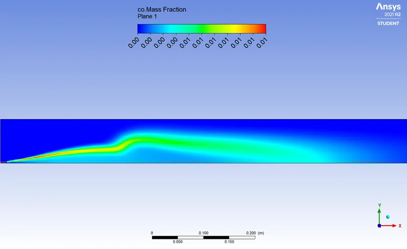
1. dp0: `CH_4 = 100 % "by mole"` & `H_2 O = 0 % "by mole"` .

1)	Residuals Graph		2)	Outlet Temperature Report
3)	CH4 mass fraction contours		4)	CH4 mass fraction chart for line probes
5)	CO mass fraction contours		6)	CO mass fraction chart for line probes
7)	CO2 mass fraction contours		8)	CO2 mass fraction chart for line probes
9)	H2O mass fraction contours		10)	H2O mass fraction chart for line probes
11)	N2 mass fraction contours		12)	N2 mass fraction chart for line probes
13)	O2 mass fraction contours		14)	O2 mass fraction chart for line probes
15)	NO mass fraction contours		16)	NO mass fraction chart for line probes
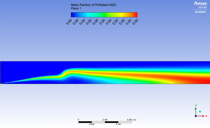
17)	NO2 mass fraction contours		18)	NO2 mass fraction chart for line probes
19)	Soot mass fraction contours		20)	Soot mass fraction chart for line probes
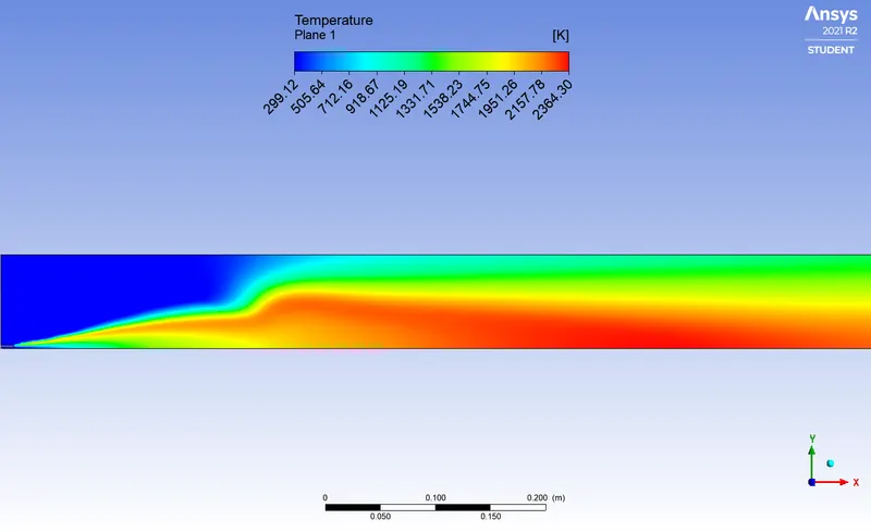
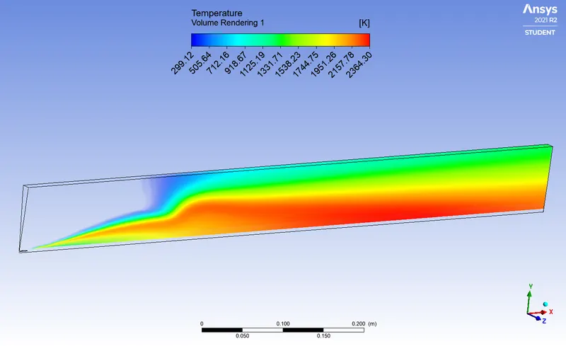
21)	Temperature contours		22)	Temperature Volume Rendering

Part 2:

Workflow:

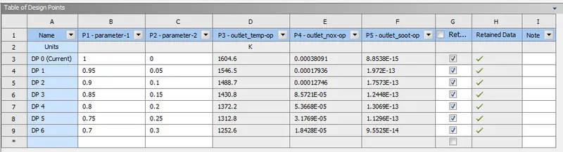
After simulating part 1 the parametric study approach is used to study the effect of water addition in the fuel varying from 5% by mole to 30 % by mole.

The required design points are defined and the same are updated through upgrade design point data.

Design Point creation and update:

Results:

1. dp1: `CH_4 = 95 % "by mole"` & `H_2 O = 5 % "by mole"` .
   
   

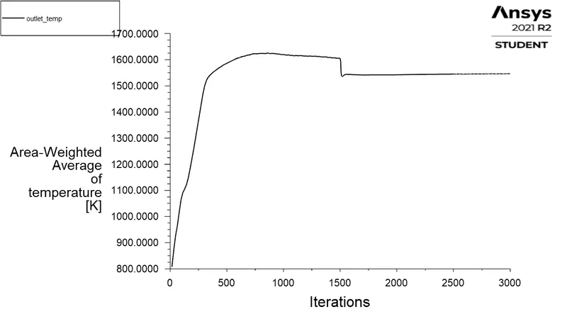
   1)	Residuals Graph		2)	Outlet Temperature Report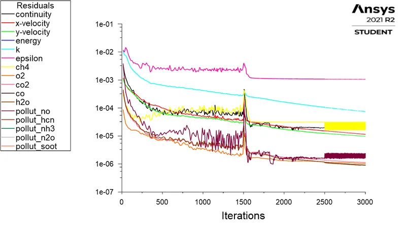
   3)	CH4 mass fraction contours		4)	CH4 mass fraction chart for line probes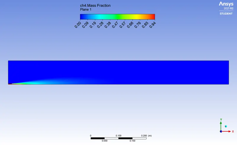
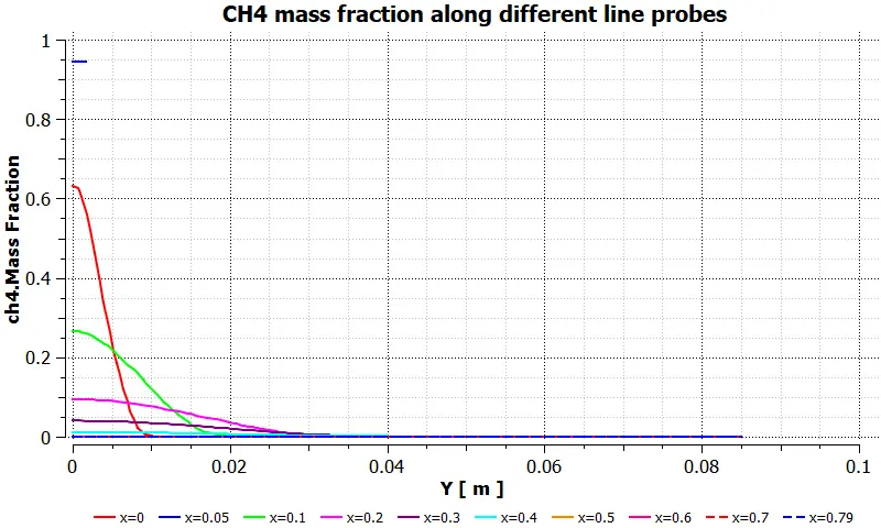
   5)	CO mass fraction contours		6)	CO mass fraction chart for line probes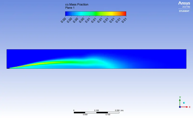
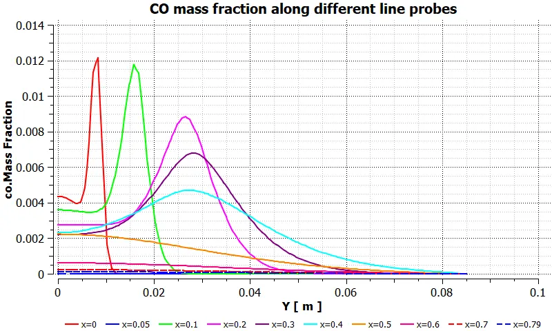
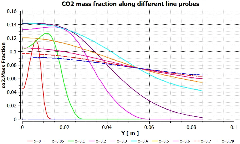
   7)	CO2 mass fraction contours		8)	CO2 mass fraction chart for line probes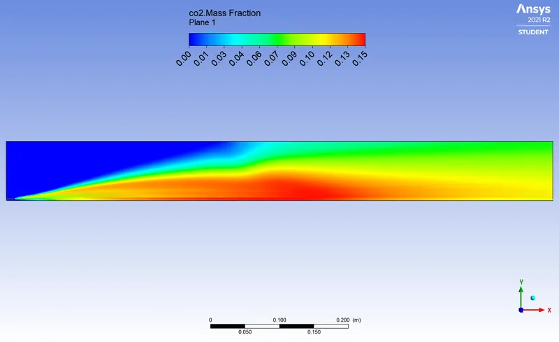
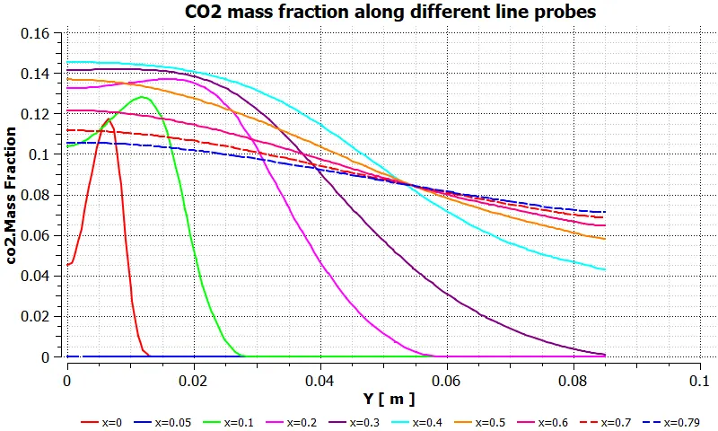
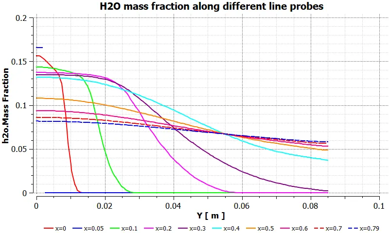
   9)	H2O mass fraction contours		10)	H2O mass fraction chart for line probes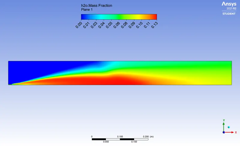
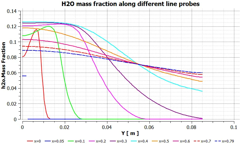
   11)	N2 mass fraction contours		12)	N2 mass fraction chart for line probes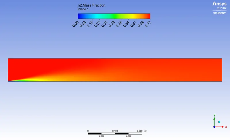
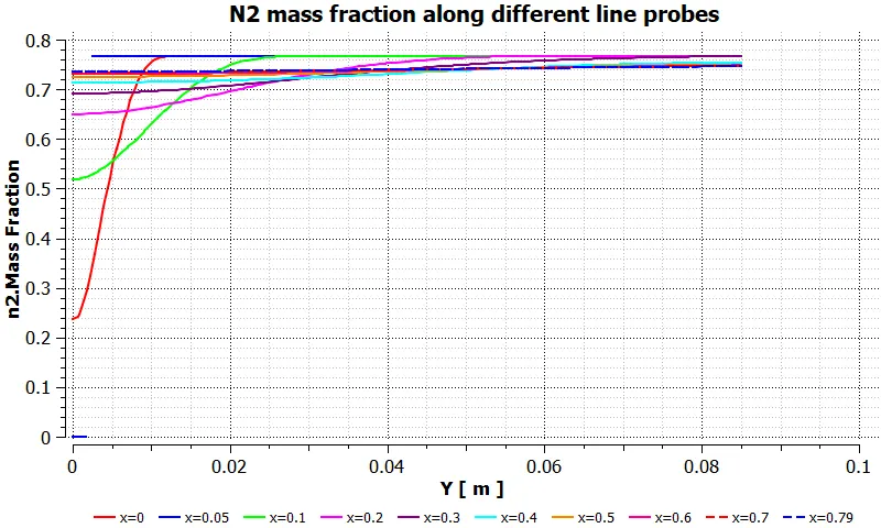
   13)	O2 mass fraction contours		14)	O2 mass fraction chart for line probes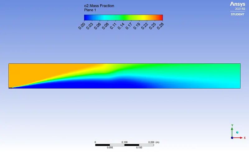
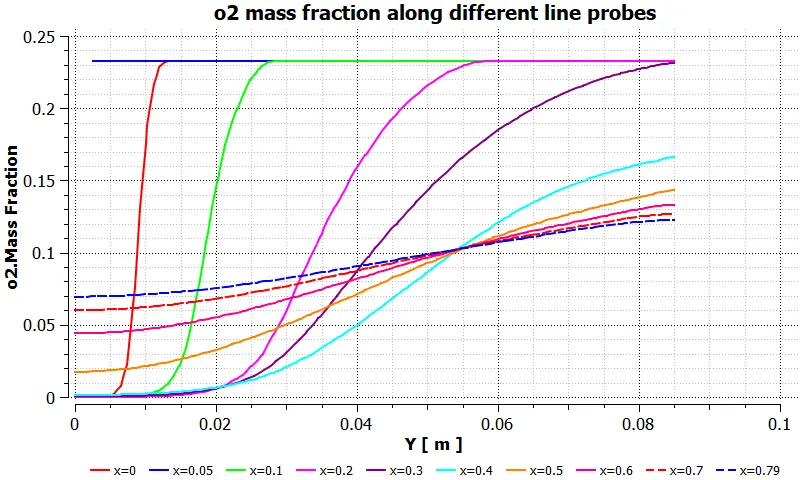
   15)	NO mass fraction contours		16)	NO mass fraction chart for line probes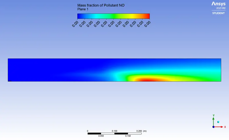
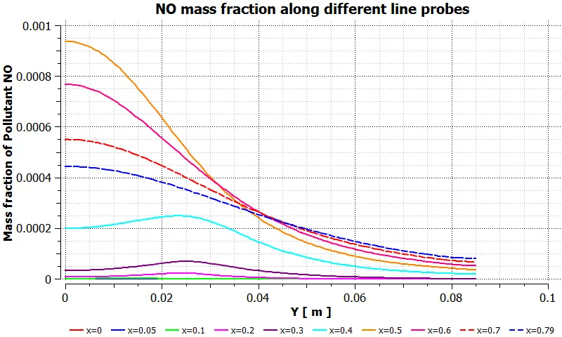
   17)	NO2 mass fraction contours		18)	NO2 mass fraction chart for line probes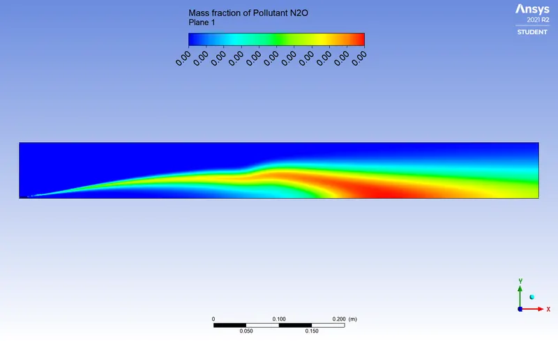
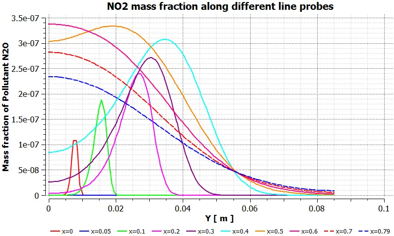
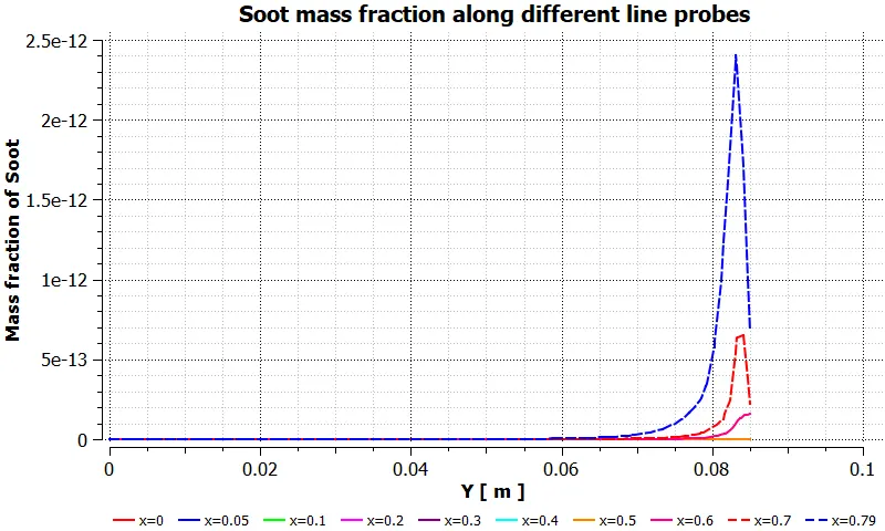
   19)	Soot mass fraction contours		20)	Soot mass fraction chart for line probes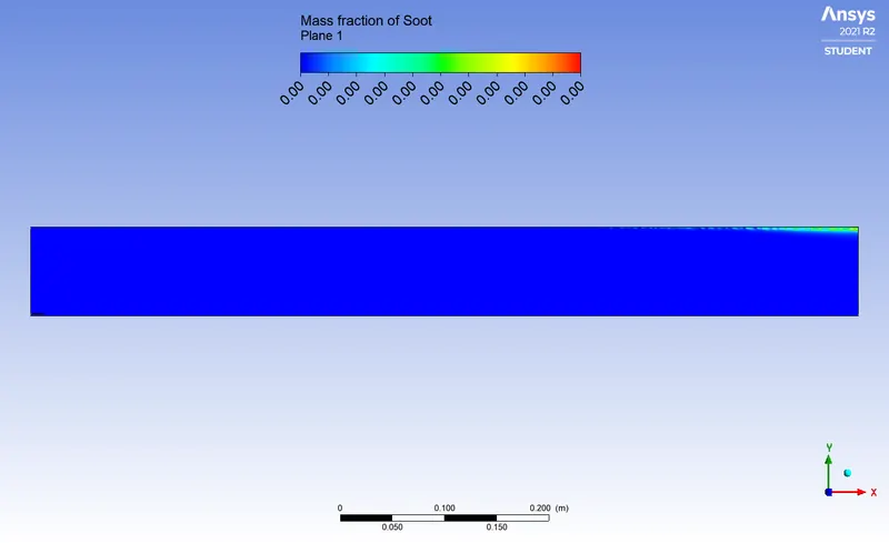
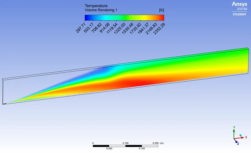
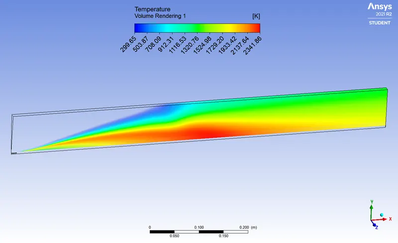
   21)	Temperature contours		22)	Temperature Volume Rendering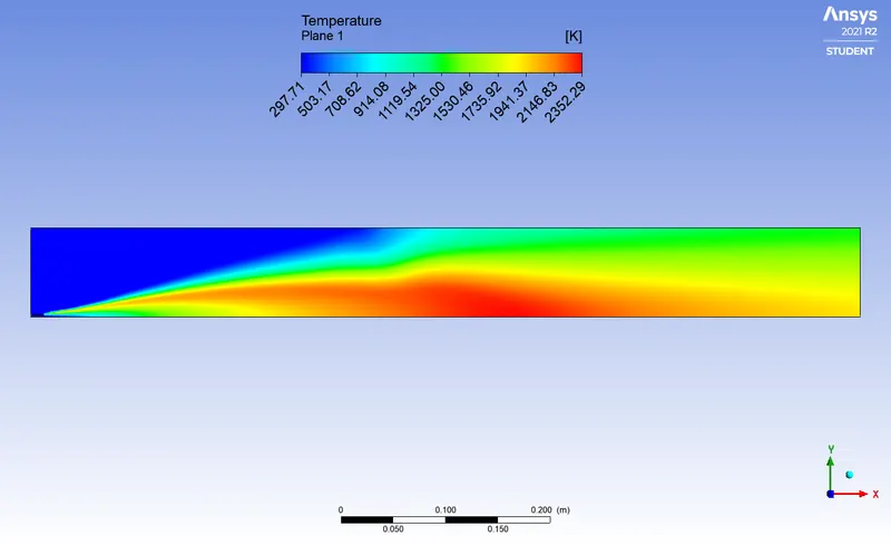

   
   
   
2. dp2: `CH_4 = 90 % "by mole"` & `H_2 O = 10 % "by mole"` .
   
   

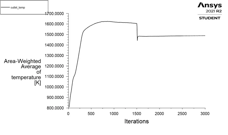
   1)	Residuals Graph		2)	Outlet Temperature Report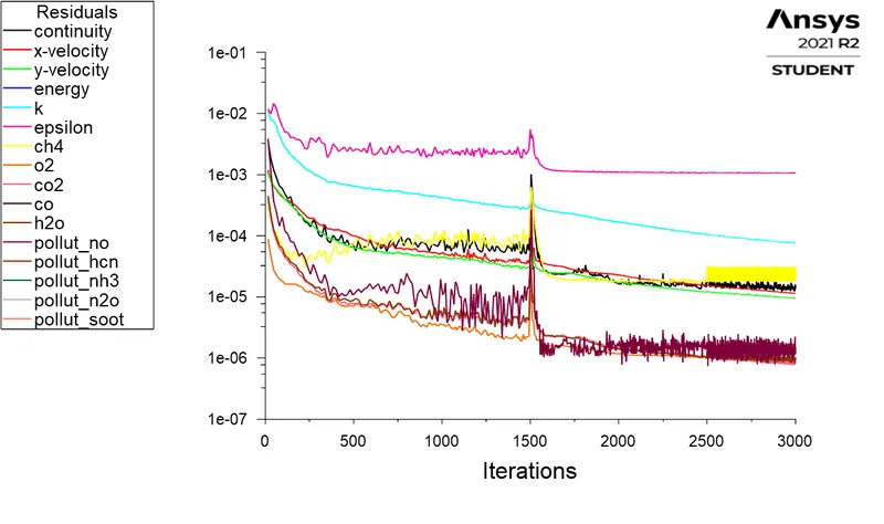
   3)	CH4 mass fraction contours		4)	CH4 mass fraction chart for line probes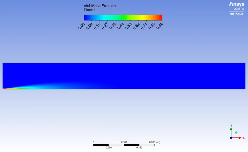
   5)	CO mass fraction contours		6)	CO mass fraction chart for line probes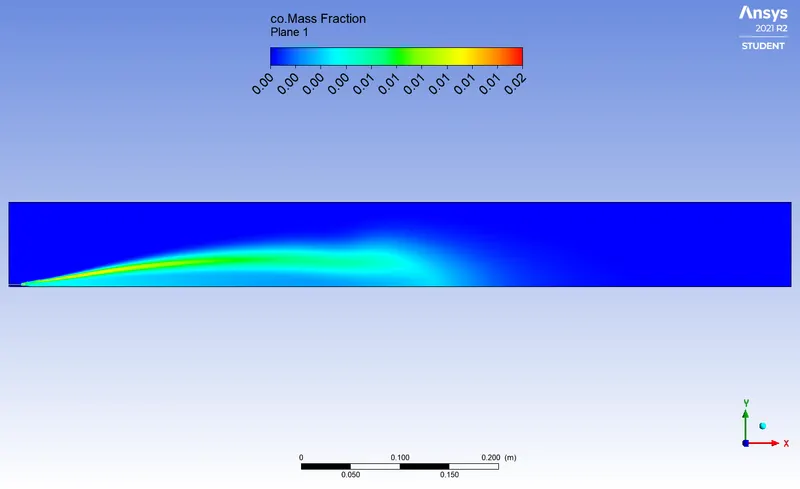
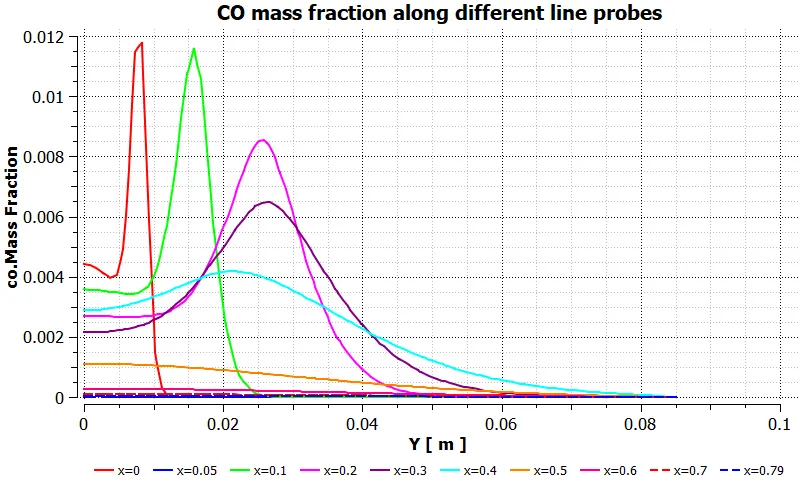
   7)	CO2 mass fraction contours		8)	CO2 mass fraction chart for line probes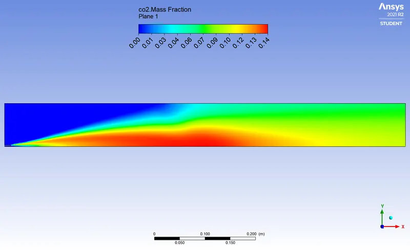
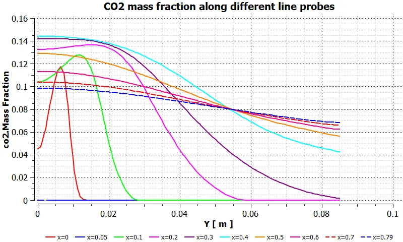
   9)	H2O mass fraction contours		10)	H2O mass fraction chart for line probes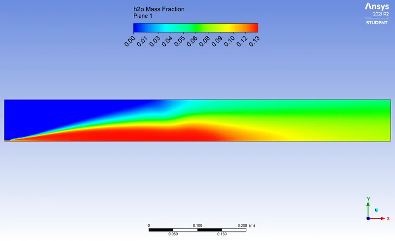
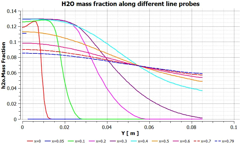
   11)	N2 mass fraction contours		12)	N2 mass fraction chart for line probes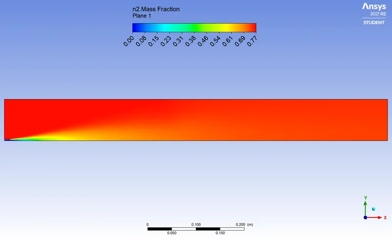
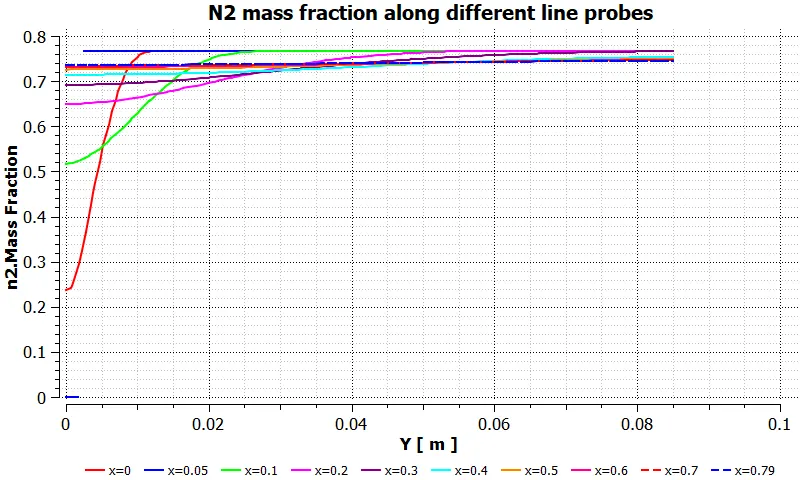
   13)	O2 mass fraction contours		14)	O2 mass fraction chart for line probes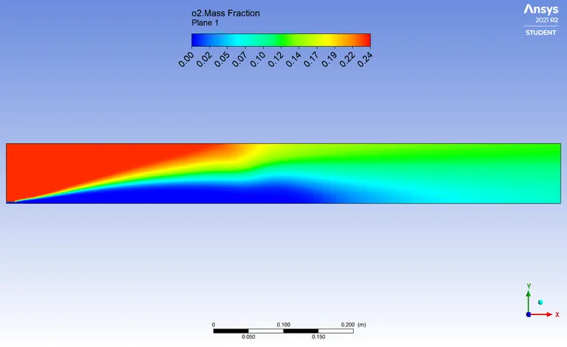
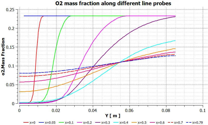
   15)	NO mass fraction contours		16)	NO mass fraction chart for line probes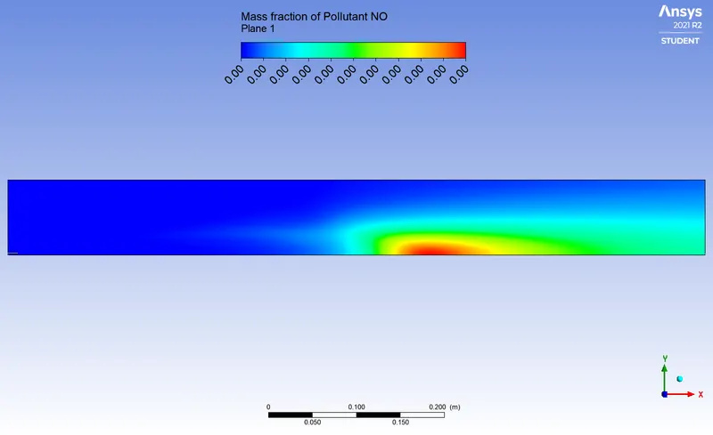
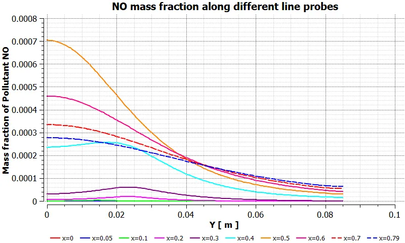
   17)	NO2 mass fraction contours		18)	NO2 mass fraction chart for line probes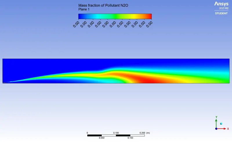
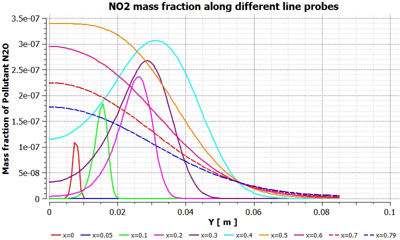
   19)	Soot mass fraction contours		20)	Soot mass fraction chart for line probes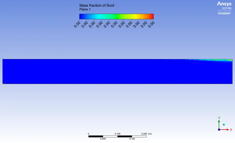
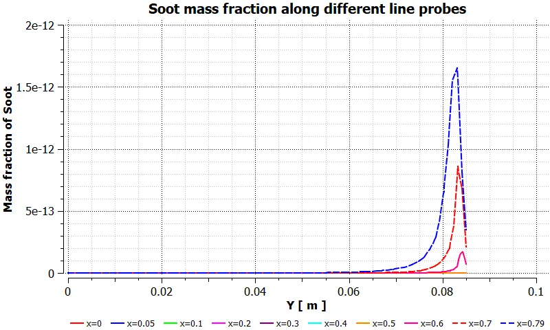
   21)	Temperature contours		22)	Temperature Volume Rendering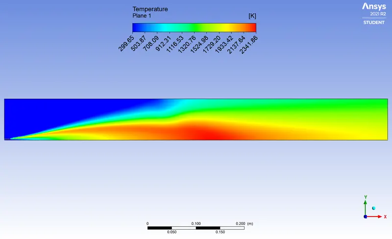

   
   
   
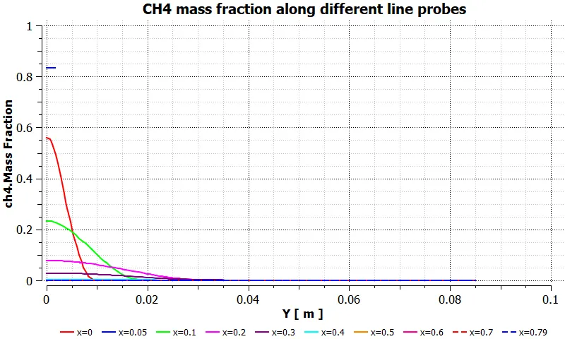
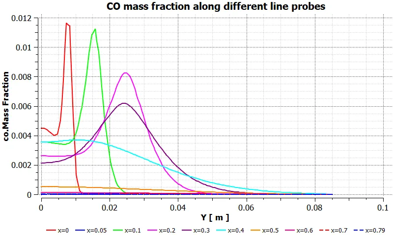
3. dp3: `CH_4 = 85 % "by mole"` & `H_2 O = 15 % "by mole"` .
   
   

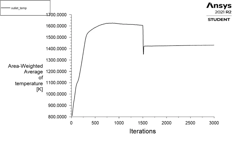
   1)	Residuals Graph		2)	Outlet Temperature Report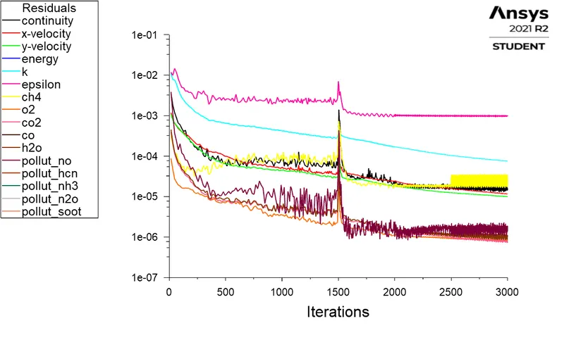
   3)	CH4 mass fraction contours		4)	CH4 mass fraction chart for line probes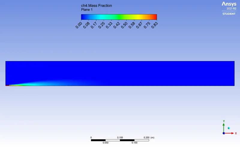
   5)	CO mass fraction contours		6)	CO mass fraction chart for line probes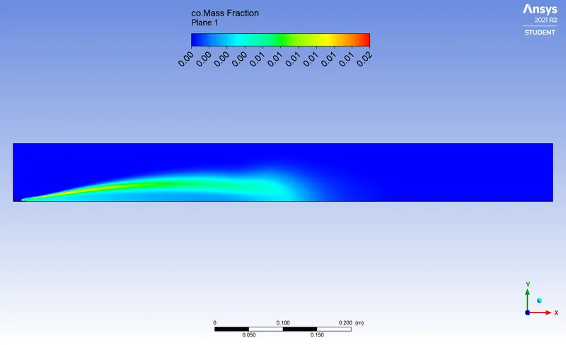
   7)	CO2 mass fraction contours		8)	CO2 mass fraction chart for line probes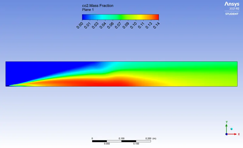
   9)	H2O mass fraction contours		10)	H2O mass fraction chart for line probes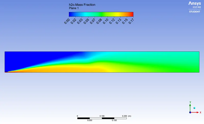
   11)	N2 mass fraction contours		12)	N2 mass fraction chart for line probes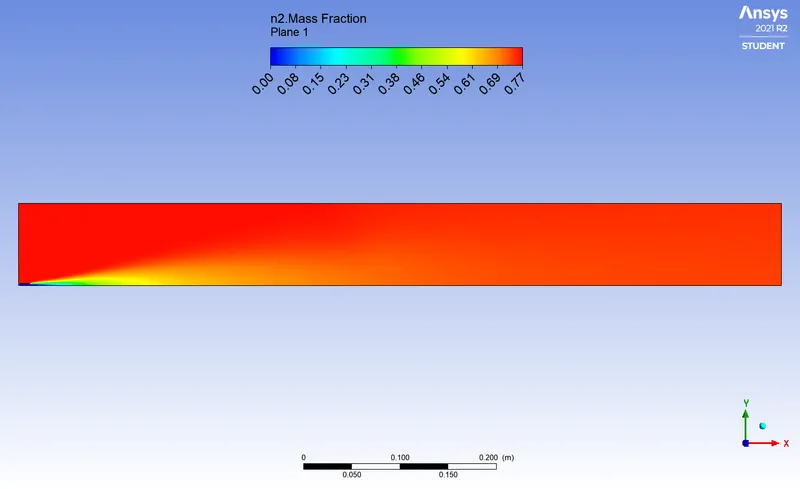
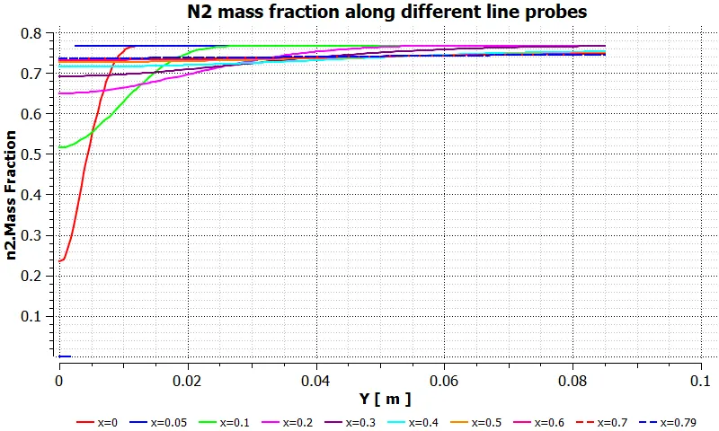
   13)	O2 mass fraction contours		14)	O2 mass fraction chart for line probes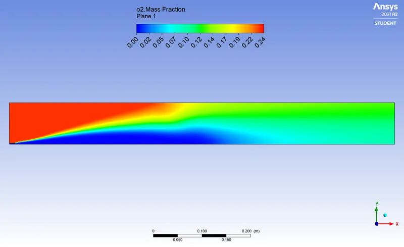
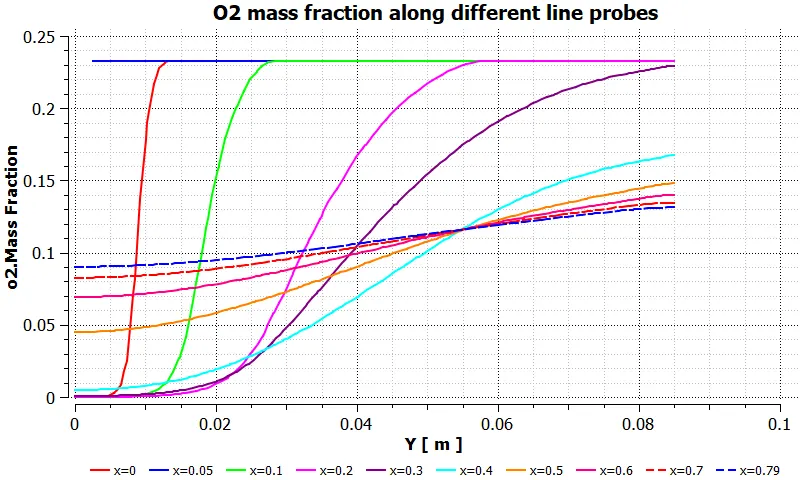
   15)	NO mass fraction contours		16)	NO mass fraction chart for line probes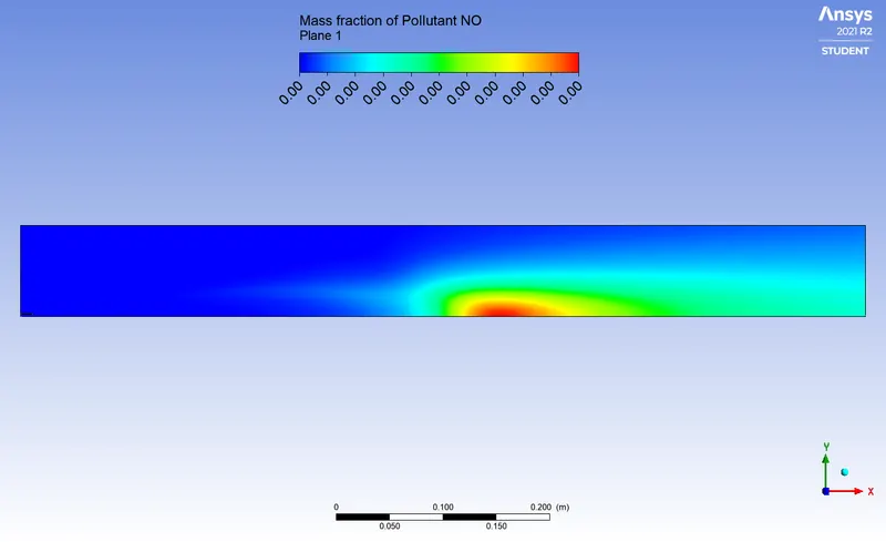
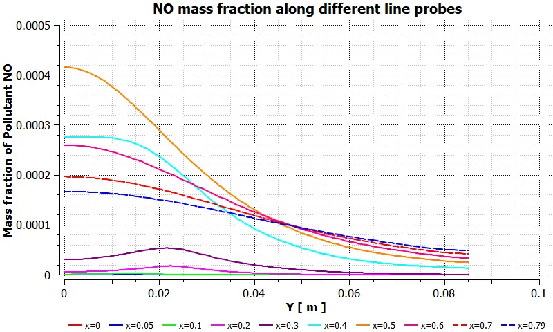
   17)	NO2 mass fraction contours		18)	NO2 mass fraction chart for line probes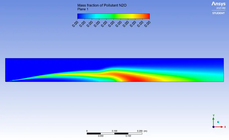
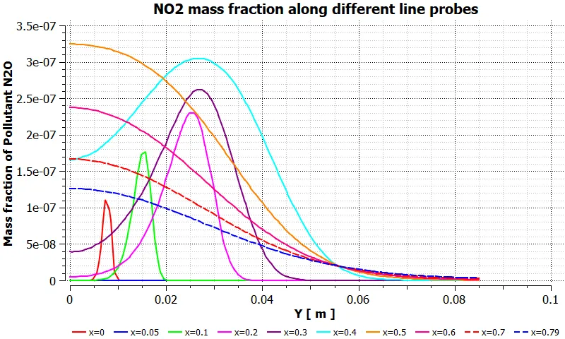
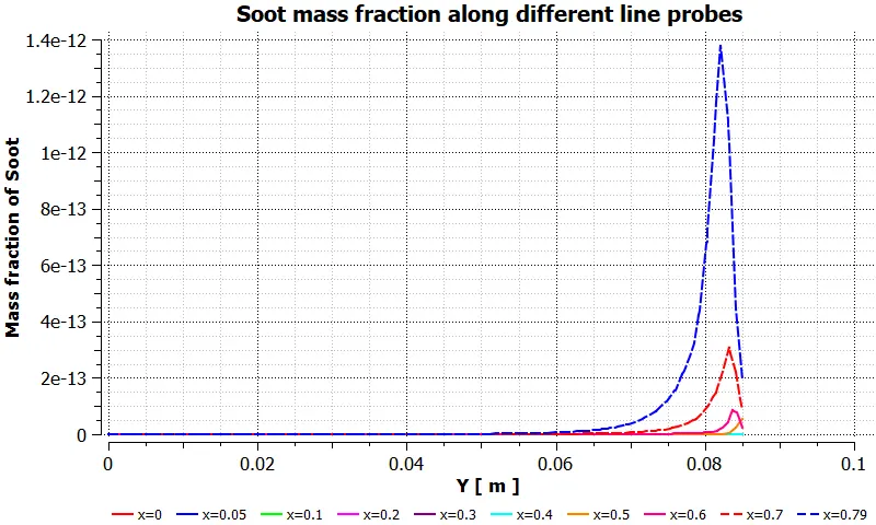
   19)	Soot mass fraction contours		20)	Soot mass fraction chart for line probes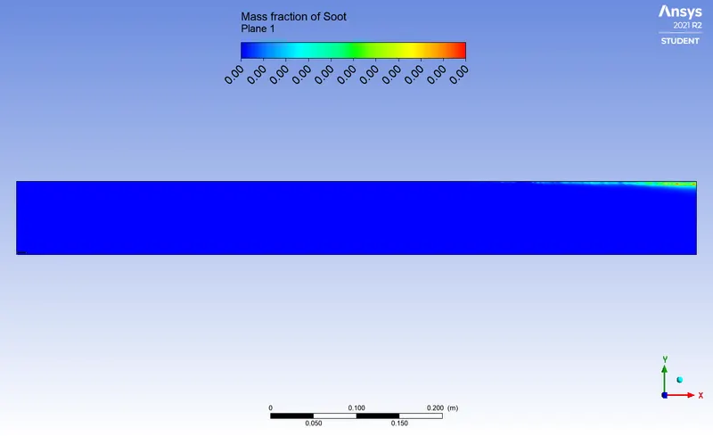
   21)	Temperature contours		22)	Temperature Volume Rendering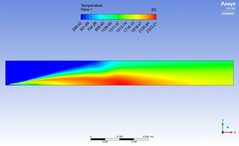

   
   
   
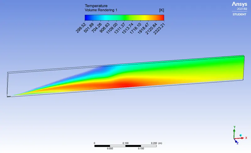
4. dp4: `CH_4 = 80 % "by mole"` & `H_2 O = 20 % "by mole"` .
   
   

   1)	Residuals Graph		2)	Outlet Temperature Report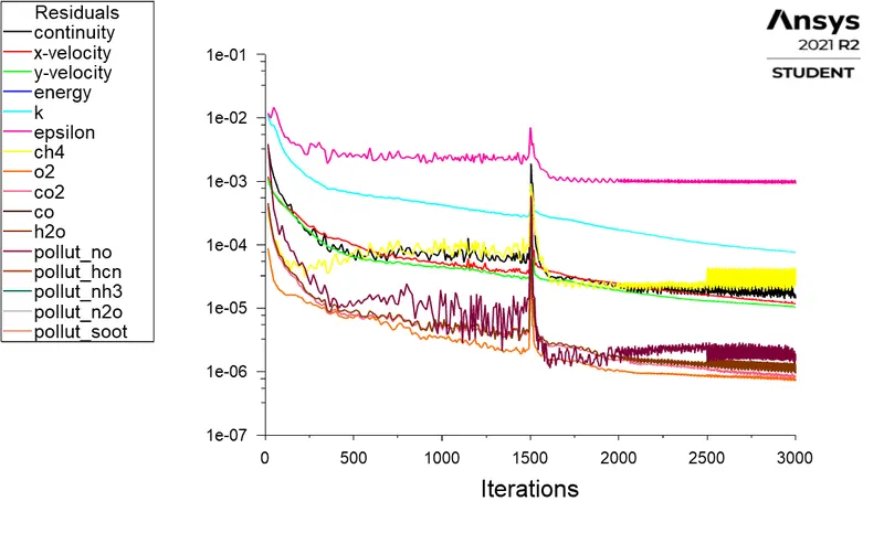
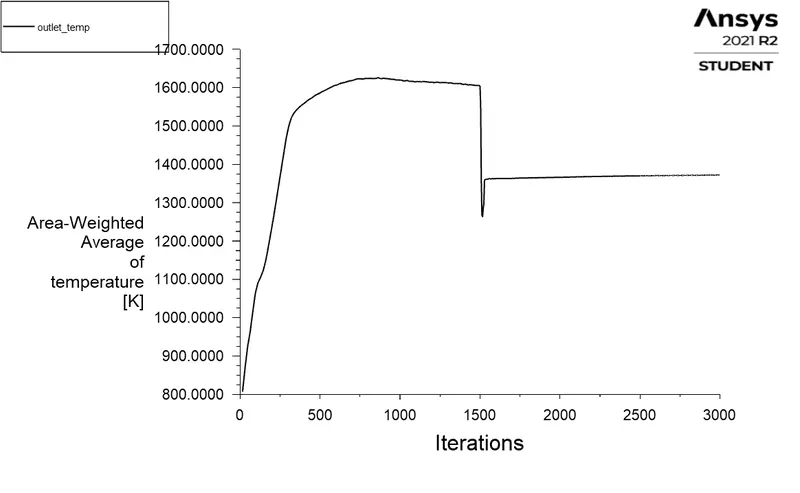
   3)	CH4 mass fraction contours		4)	CH4 mass fraction chart for line probes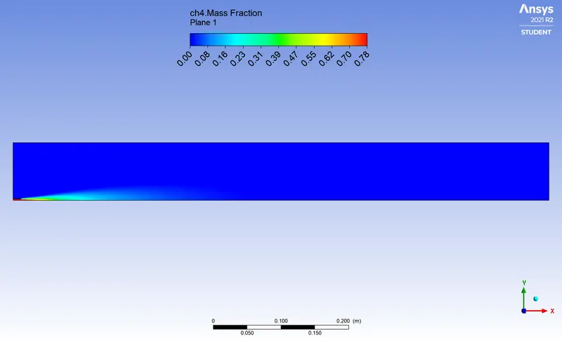
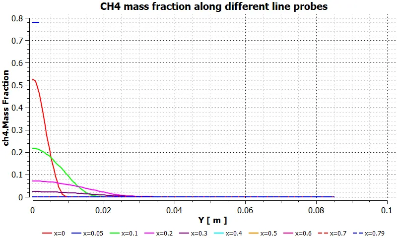
   5)	CO mass fraction contours		6)	CO mass fraction chart for line probes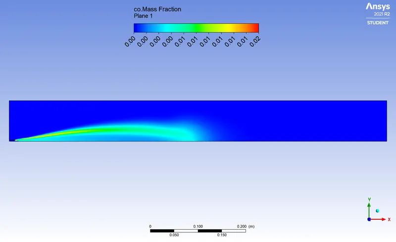
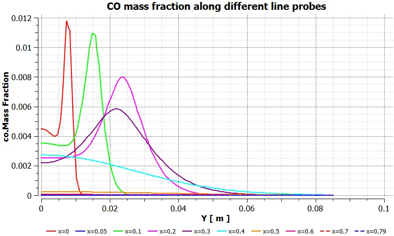
   7)	CO2 mass fraction contours		8)	CO2 mass fraction chart for line probes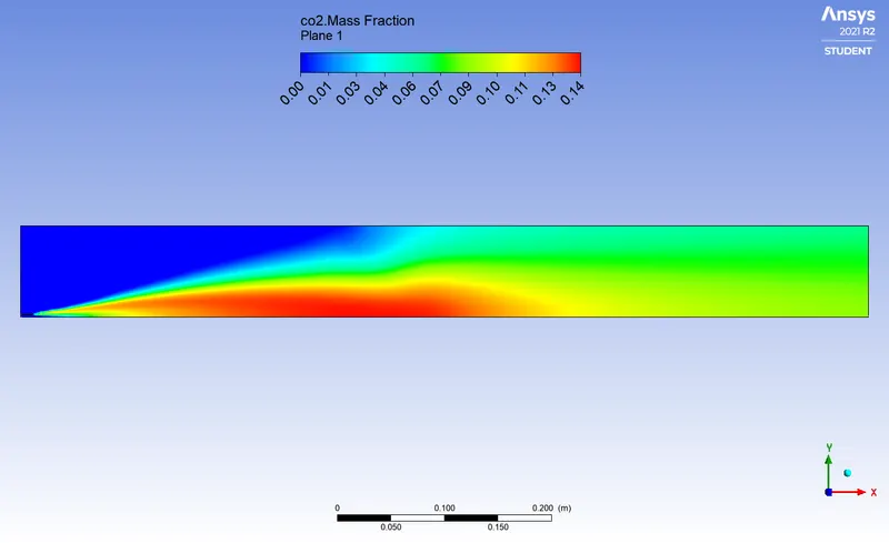
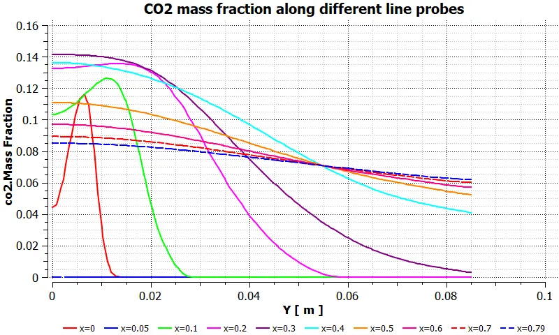
   9)	H2O mass fraction contours		10)	H2O mass fraction chart for line probes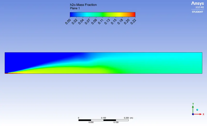
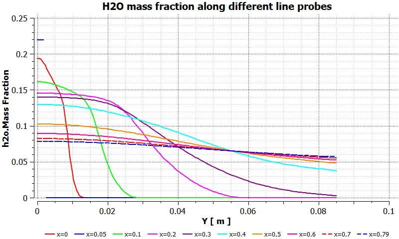
   11)	N2 mass fraction contours		12)	N2 mass fraction chart for line probes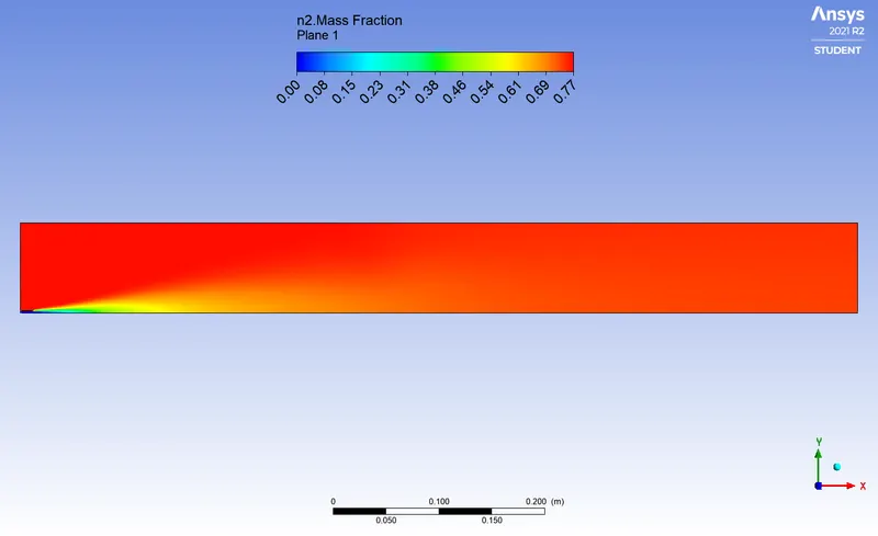
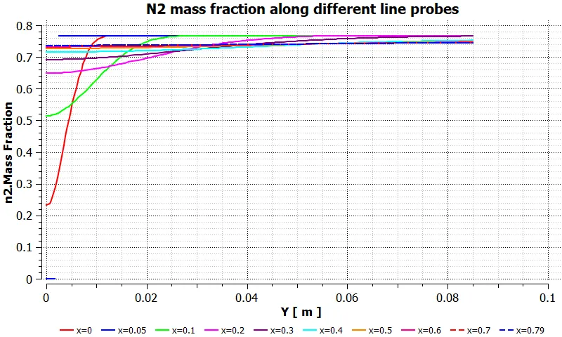
   13)	O2 mass fraction contours		14)	O2 mass fraction chart for line probes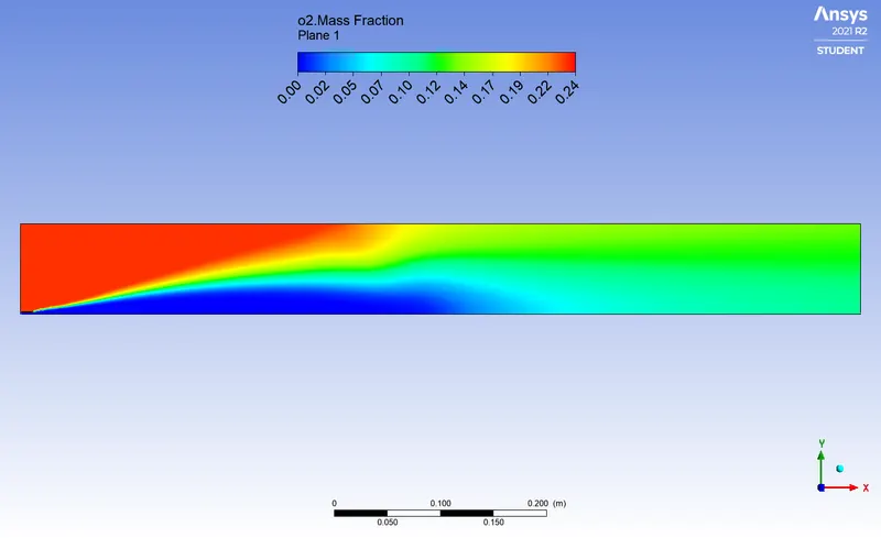
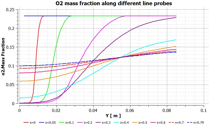
   15)	NO mass fraction contours		16)	NO mass fraction chart for line probes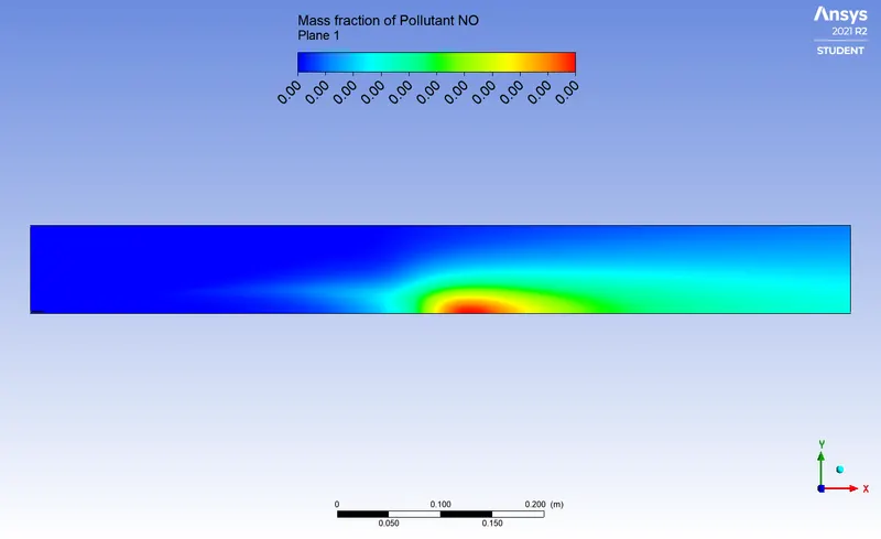
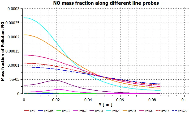
   17)	NO2 mass fraction contours		18)	NO2 mass fraction chart for line probes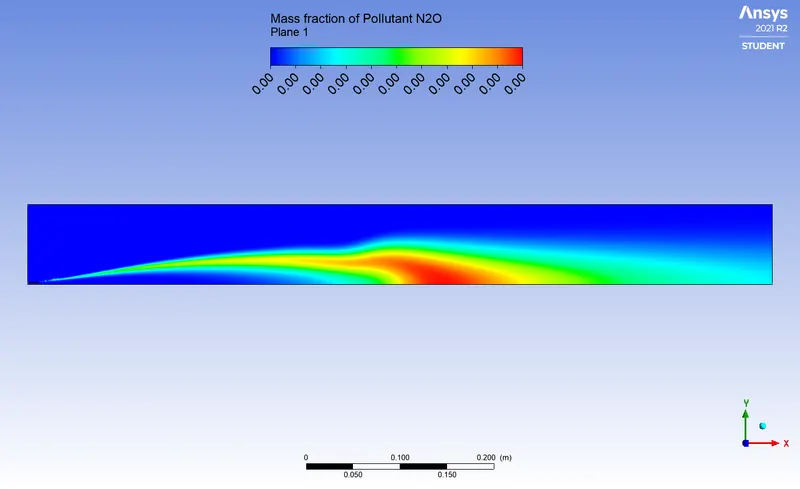
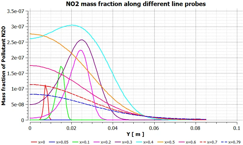
   19)	Soot mass fraction contours		20)	Soot mass fraction chart for line probes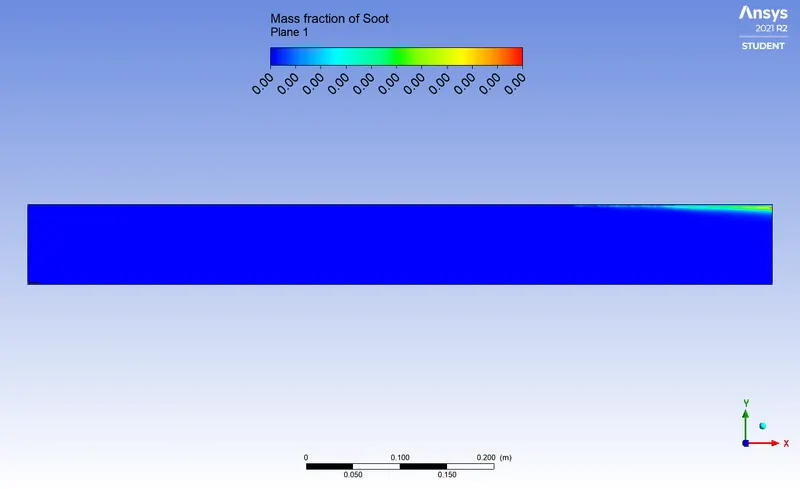
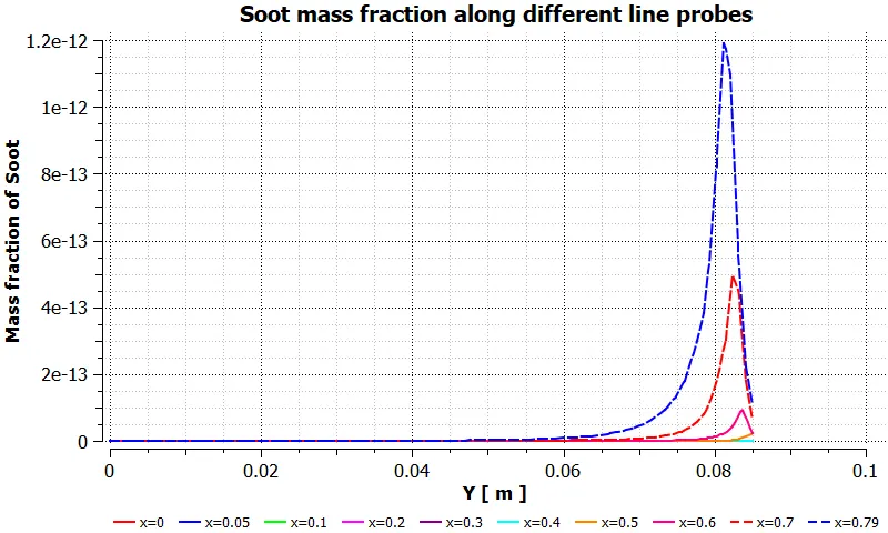
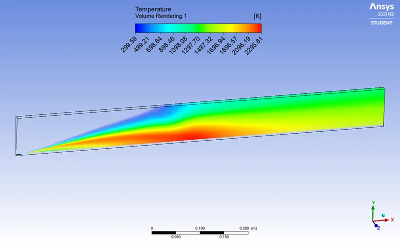
   21)	Temperature contours		22)	Temperature Volume Rendering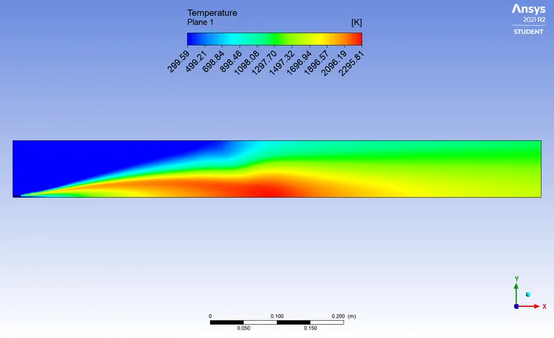

   
   
   
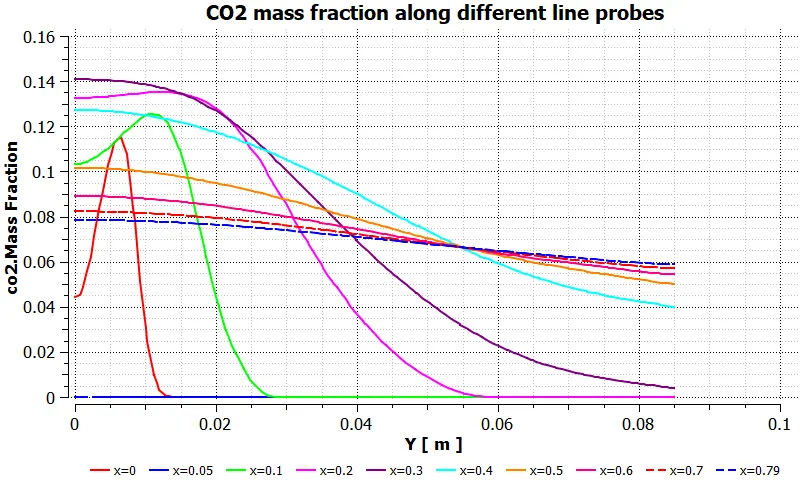
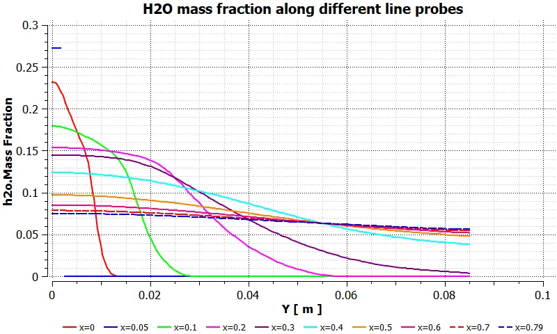
5. dp5: `CH_4 = 75 % "by mole"` & `H_2 O = 25 % "by mole"` .
   
   

   1)	Residuals Graph		2)	Outlet Temperature Report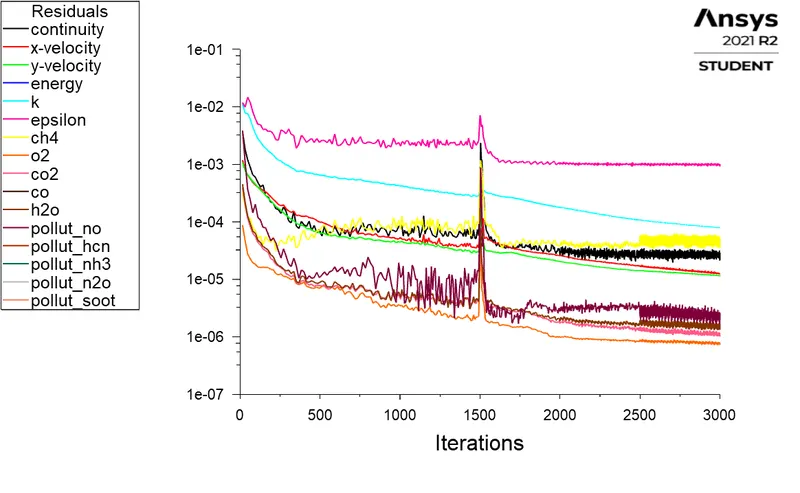
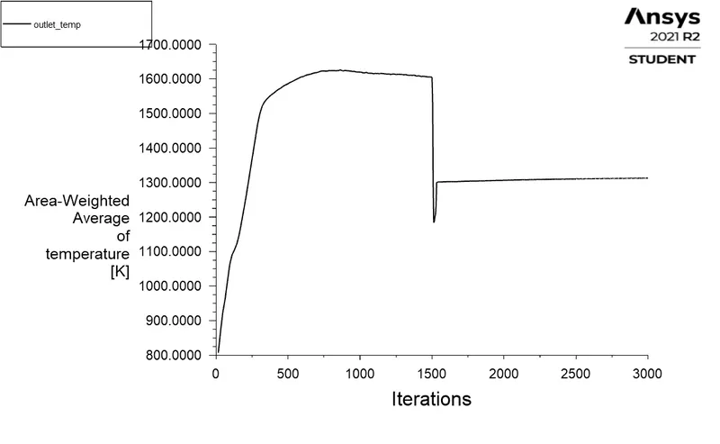
   3)	CH4 mass fraction contours		4)	CH4 mass fraction chart for line probes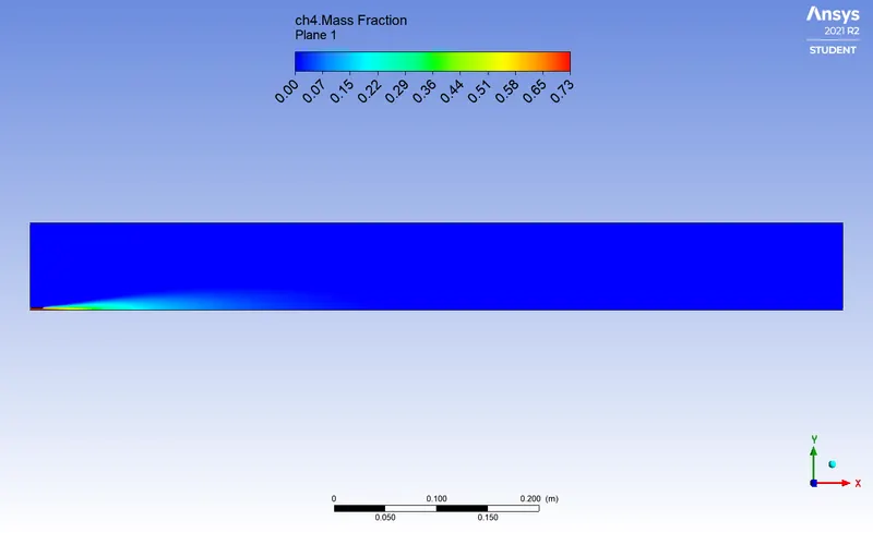
   5)	CO mass fraction contours		6)	CO mass fraction chart for line probes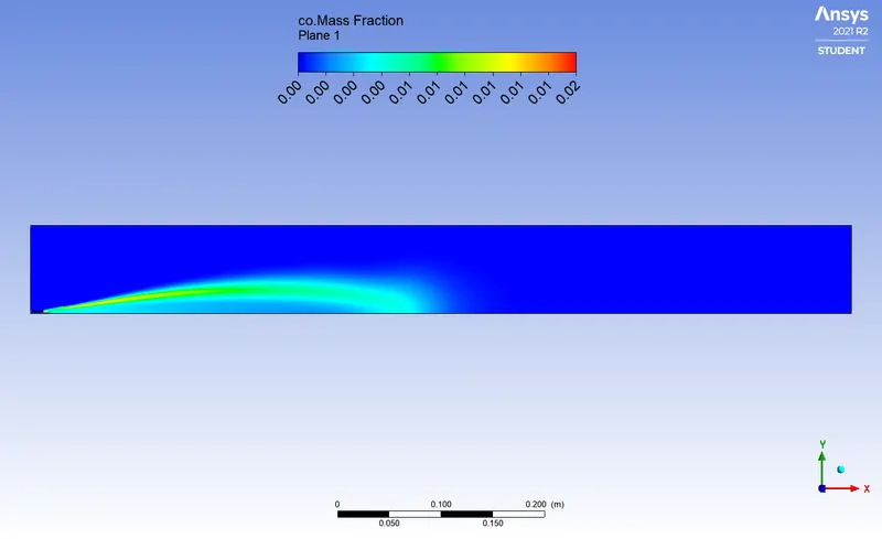
   7)	CO2 mass fraction contours		8)	CO2 mass fraction chart for line probes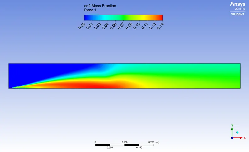
   9)	H2O mass fraction contours		10)	H2O mass fraction chart for line probes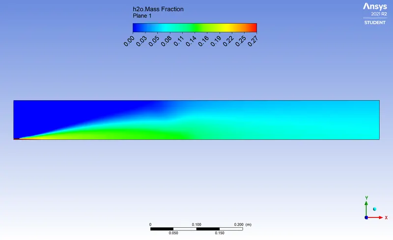
   11)	N2 mass fraction contours		12)	N2 mass fraction chart for line probes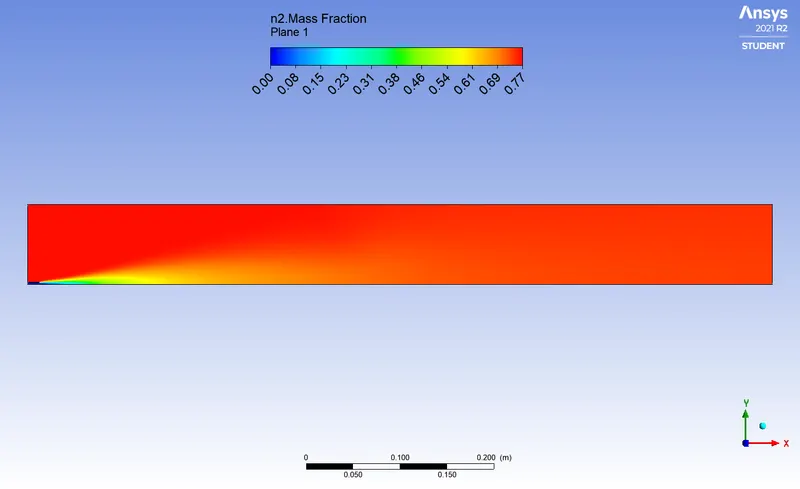
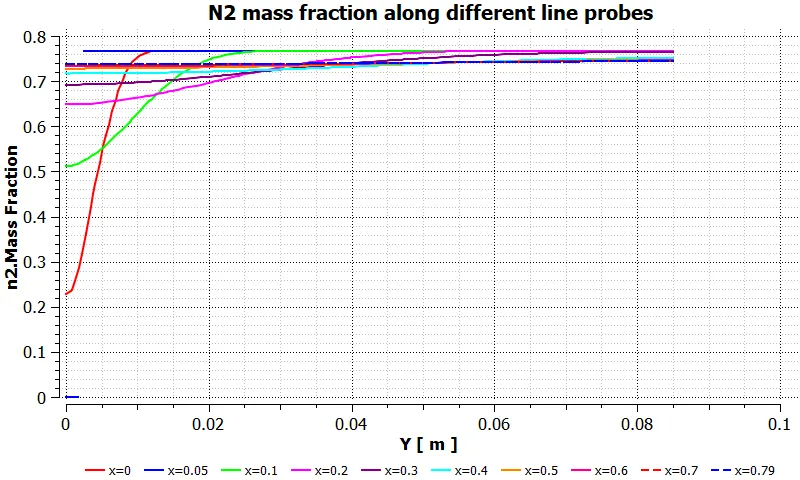
   13)	O2 mass fraction contours		14)	O2 mass fraction chart for line probes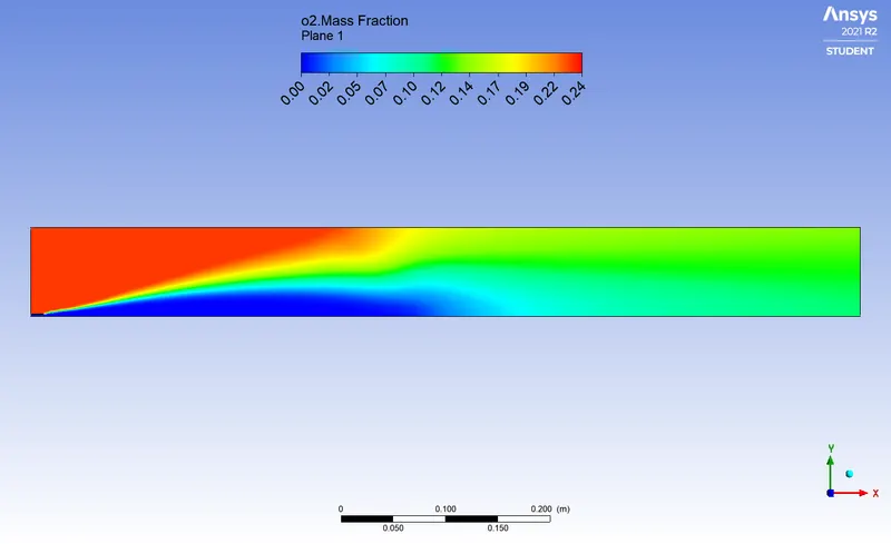
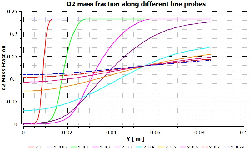
   15)	NO mass fraction contours		16)	NO mass fraction chart for line probes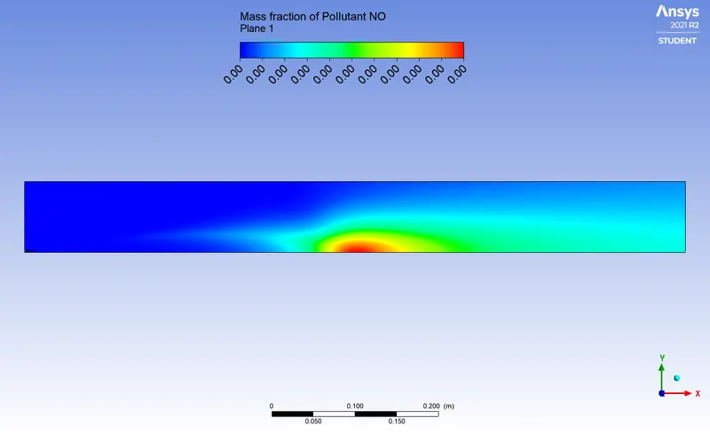
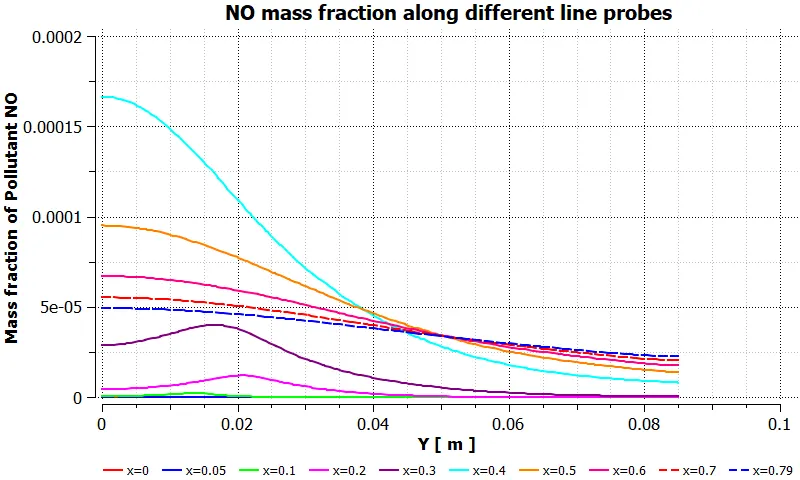
   17)	NO2 mass fraction contours		18)	NO2 mass fraction chart for line probes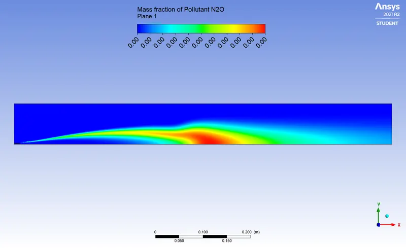
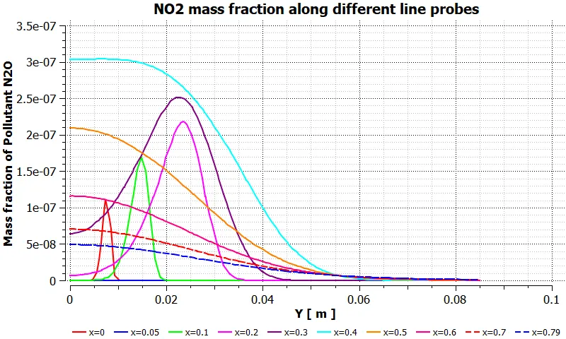
   19)	Soot mass fraction contours		20)	Soot mass fraction chart for line probes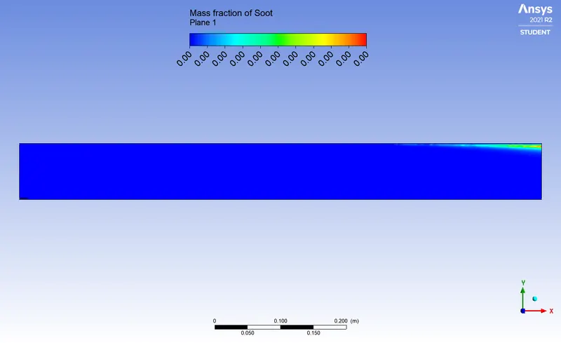
   21)	Temperature contours		22)	Temperature Volume Rendering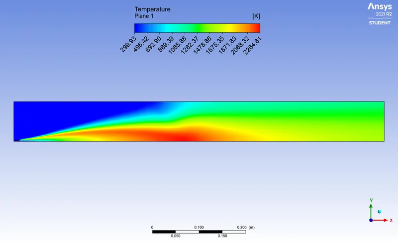

   
   
   
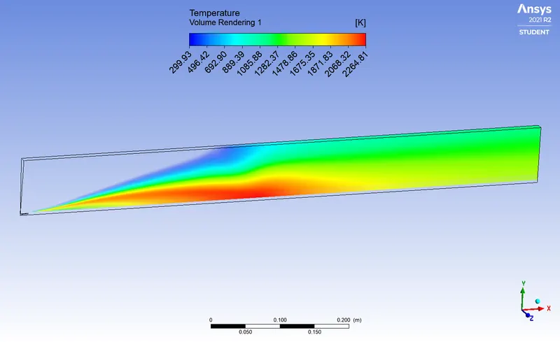
6. dp6: `CH_4 = 70 % "by mole"` & `H_2 O = 30 % "by mole" `.
   
   

   1)	Residuals Graph		2)	Outlet Temperature Report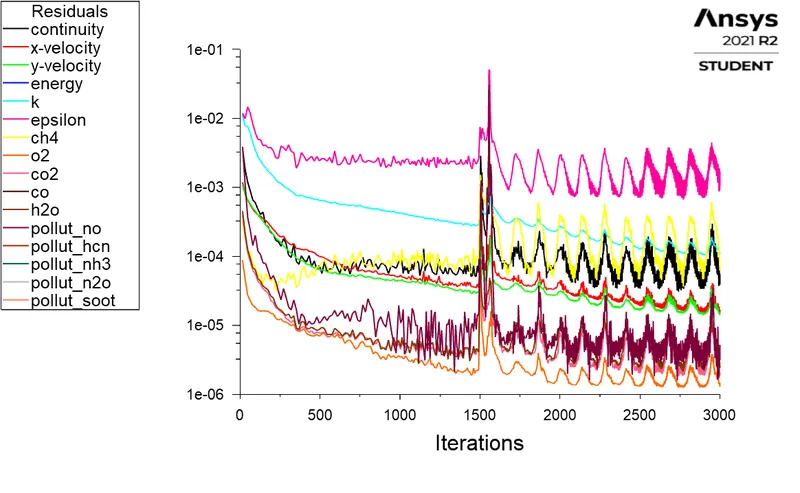
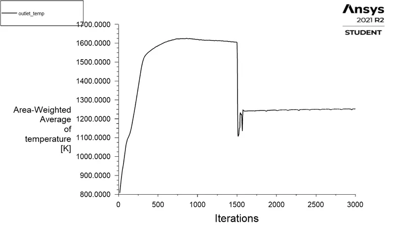
   3)	CH4 mass fraction contours		4)	CH4 mass fraction chart for line probes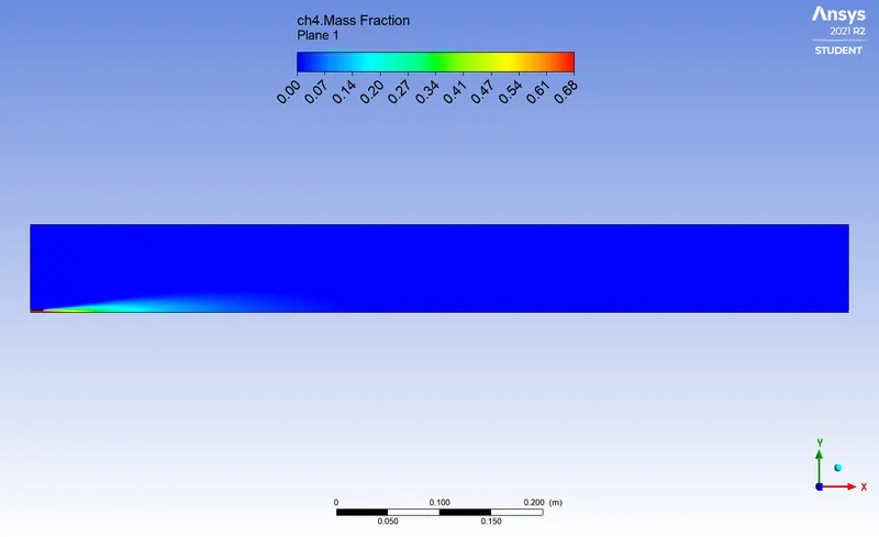
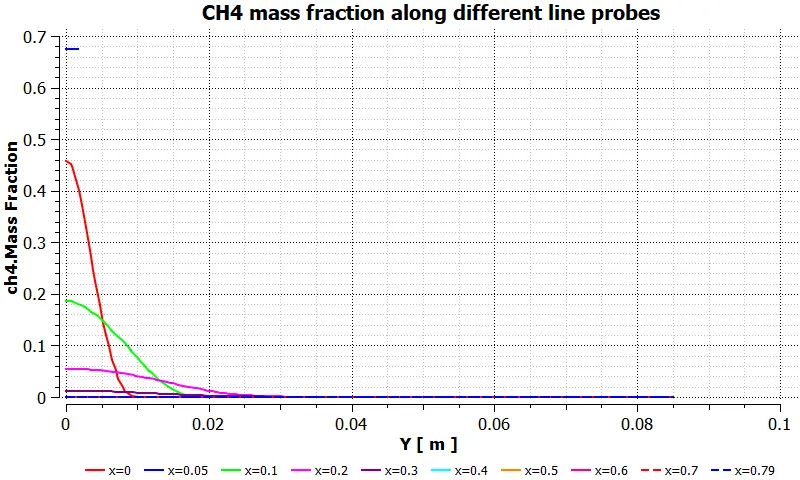
   5)	CO mass fraction contours		6)	CO mass fraction chart for line probes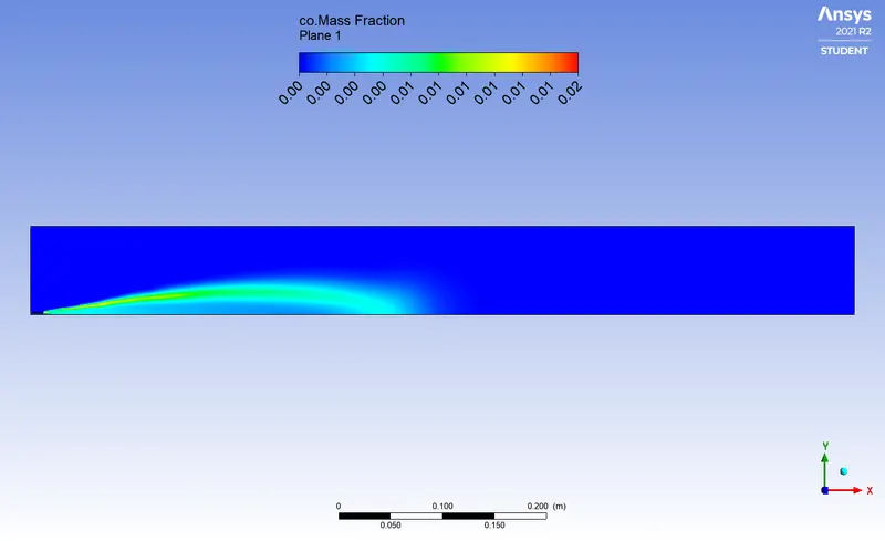
   7)	CO2 mass fraction contours		8)	CO2 mass fraction chart for line probes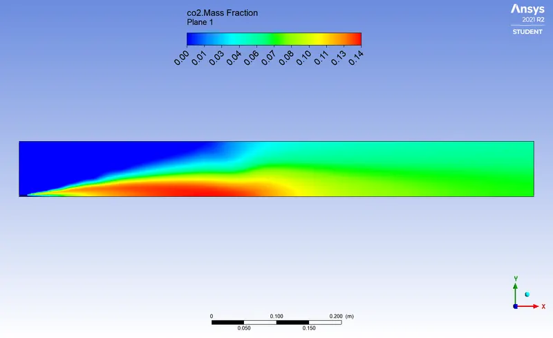
   9)	H2O mass fraction contours		10)	H2O mass fraction chart for line probes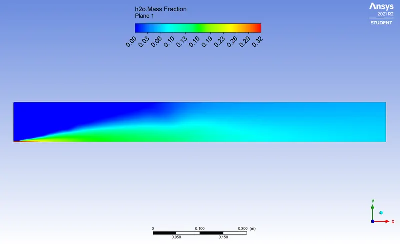
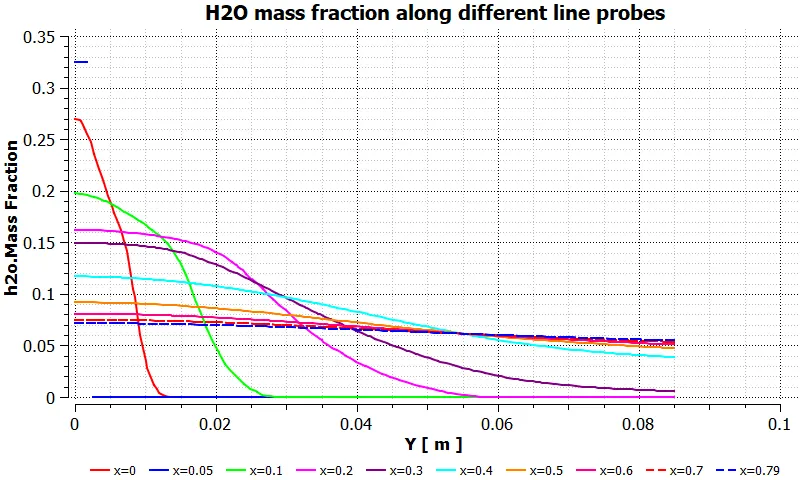
   11)	N2 mass fraction contours		12)	N2 mass fraction chart for line probes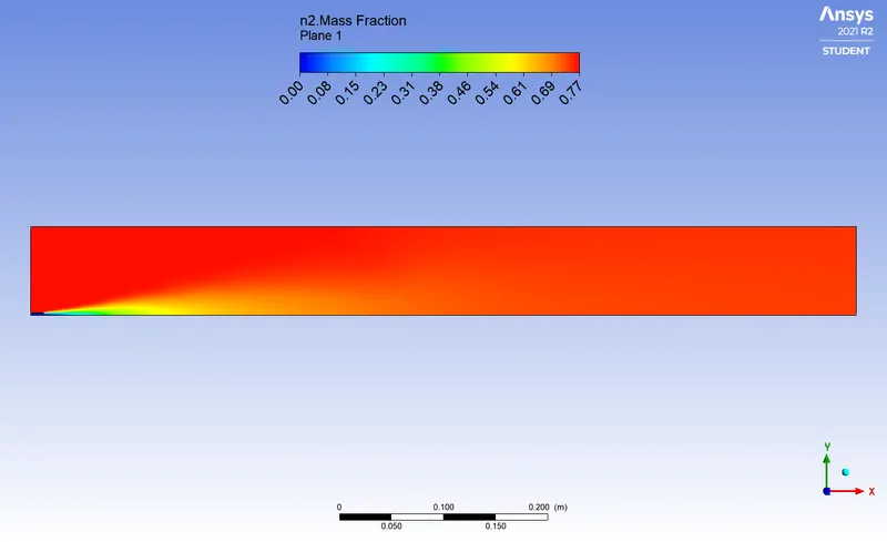
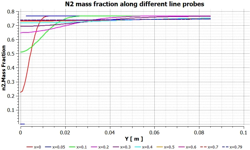
   13)	O2 mass fraction contours		14)	O2 mass fraction chart for line probes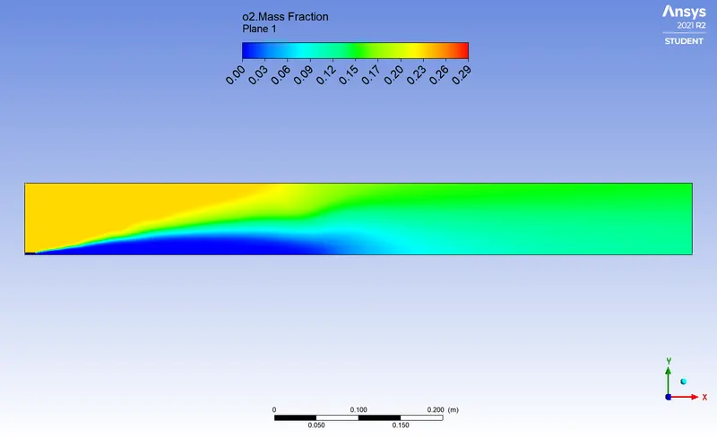
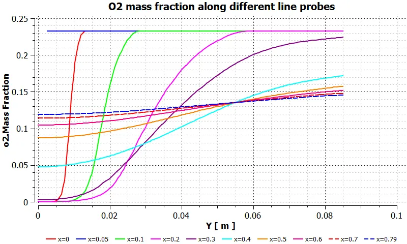
   15)	NO mass fraction contours		16)	NO mass fraction chart for line probes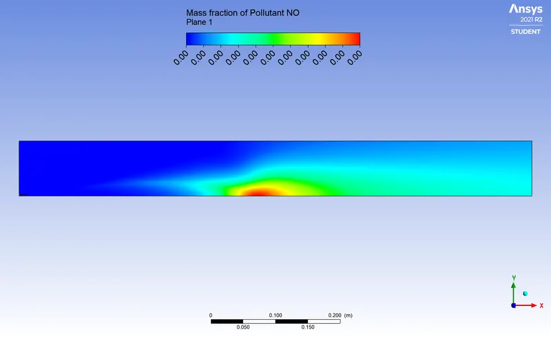
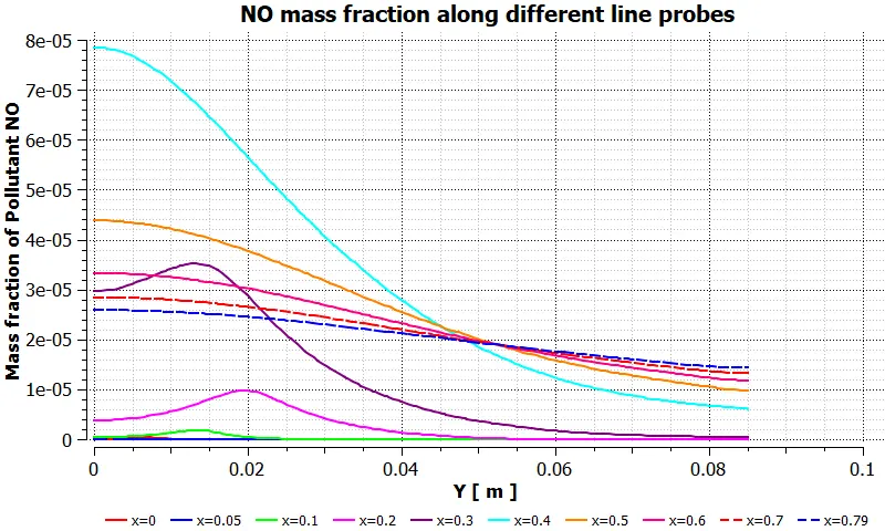
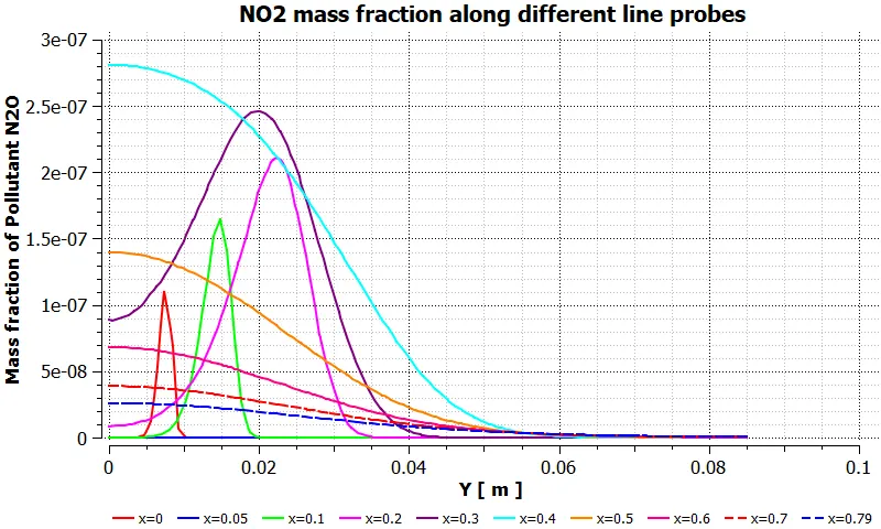
   17)	NO2 mass fraction contours		18)	NO2 mass fraction chart for line probes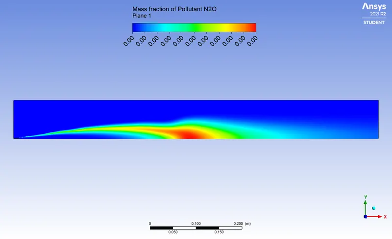
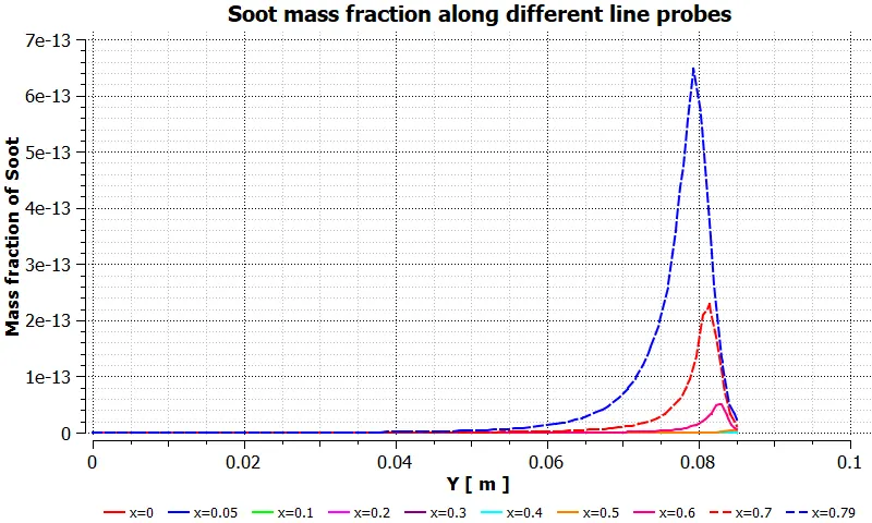
   19)	Soot mass fraction contours		20)	Soot mass fraction chart for line probes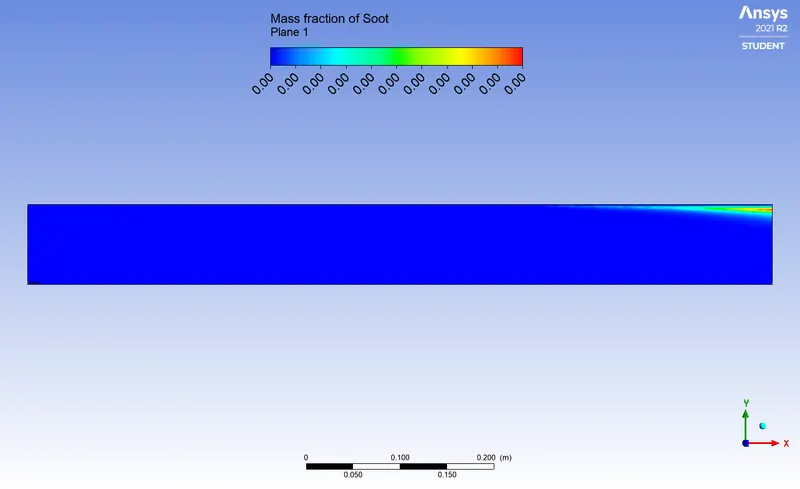
   21)	Temperature contours		22)	Temperature Volume Rendering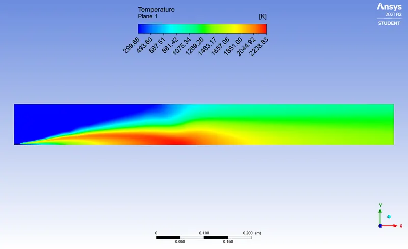

   
   
   

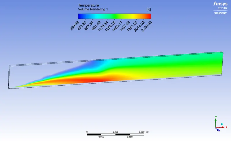
Observation Table and Graphs: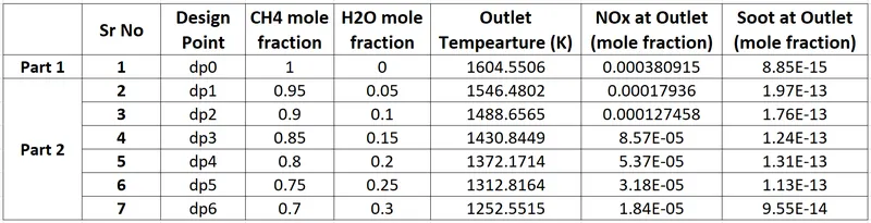

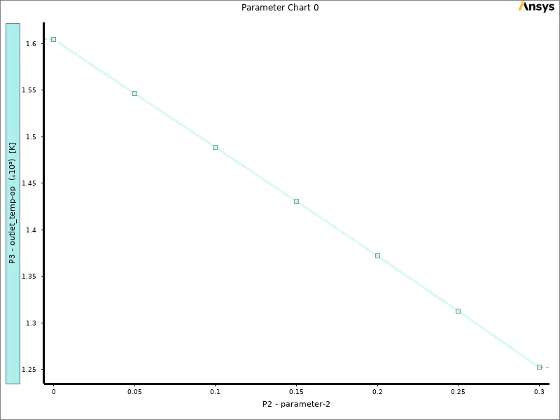
Graph I: Outlet Temperature Vs H2O mole fraction (parameter-2)

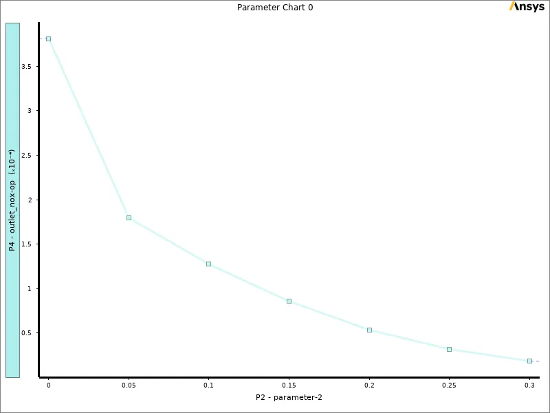
Graph II: NOx mole fraction at Outlet Vs H2O mole fraction (parameter-2)

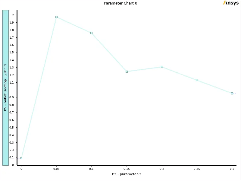
Graph III: Soot mole fraction at outlet Vs H2O mole fraction (parameter-2)

Conclusions:

1. Mass fractions of the species CO2, H2O, CH4, N2, O2, NOx emissions & Soot formation at the different line probes are plotted and observed. The trends are inline with the input variations made regarding water content in the fuel.

2. From the results, observation tables and the graphs above it can be concluded that the addition of water into fuel decreases the overall temperature at the outlet.

3. As the outlet temperature decreases the NOx levels at the outlet of the combustor should be decreased as the high temperature influences the NOx formation. The same trend can be observed in the graph of NOx level at outlet versus water content in the fuel.

4. The graph Soot level at the outlet versus the water content in the fuel shows that the soot level increases initially with increase in the water content but as the water content in fuel increases further the soot level decreases.

   Thus the combustion analysis of natural gas (`CH_4`) is done using Ansys Fluent.