Week 10: Project 1 - FULL HYDRO case set up (PFI)

Aim: - To run a Full-Hydro simulation on an IC engine.

Objective: -

1. Discuss the need of wall heat transfer model. why can't we predict wall temperature from CFD simulation?
2. To prepare the surface and flag the boundary and setup a Full-hydro case.
3. To Calculate combustion effeciency, Compression Ratio and use the engine performance calculator, to determine the power and torque for this engine.
4. Discuss the the significance of ca10, ca50 and ca90. Create an animation of Full-hydro and mesh with respect to time.

Introduction: -

Model of IC engine –

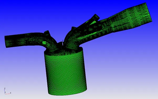
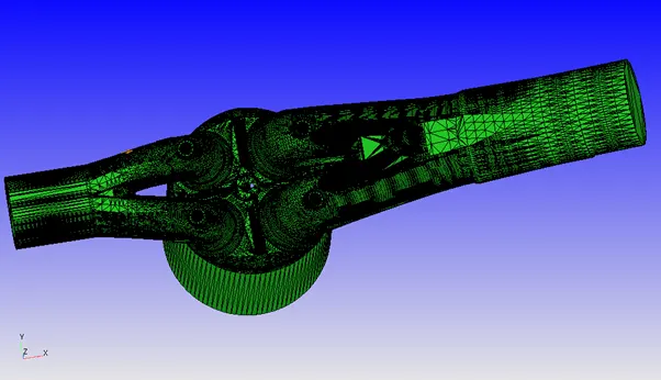
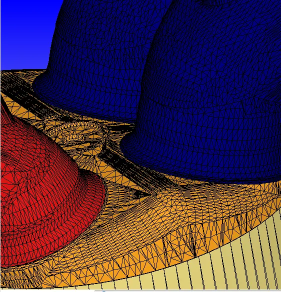
Diagnosing the model following problems are encountered

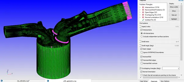
Steps to clean and prepare the geometry

1. Normal orientation is flipped for one triangle and propagated using transform tab in geometry dock. Normal orientation is resolved along with few overlapping triangles.
2. Open edges are patched and overlapping triangles are deleted.
3. Intersection triangles are due to valve intersecting the port. To remove this Valves are flagged and translated along the normal of the valve.

During the flagging of valves and ports the ring triangles should belong to the non-translating boundary to avoid alignment error.

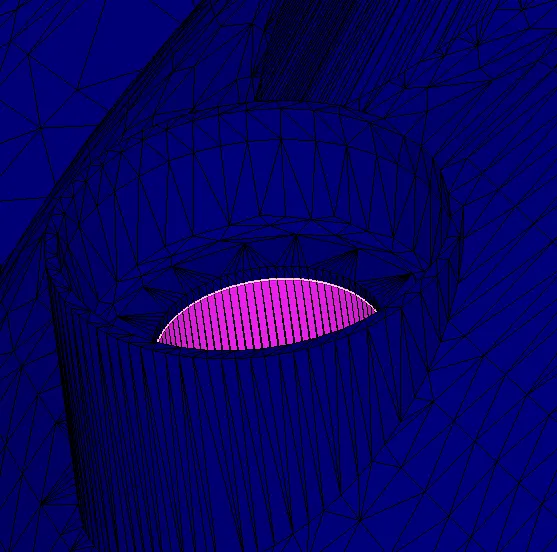
The boundary at intake port and cylinder should be appropriate to avoid alignment error due to disconnect triangles.

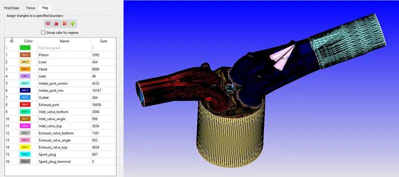
Boundary –

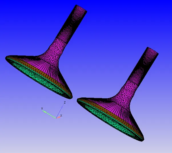
Inlet Valve flags-

Exhaust Valve flags –

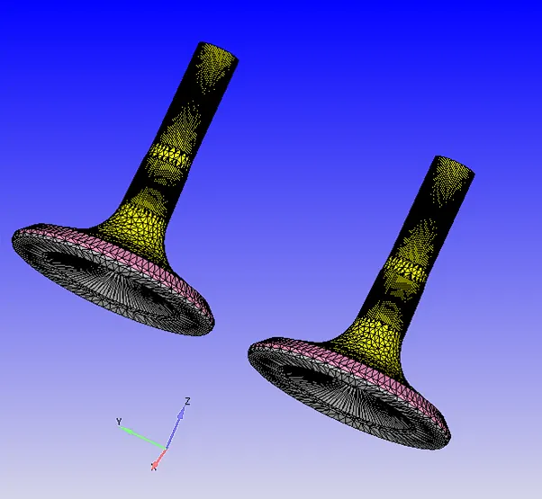
Valves are divided into 3 parts namely – Top, angle and Bottom as different boundary of the valve belongs to different regions and for putting mesh refinements on angle boundary.

Case Setup: -

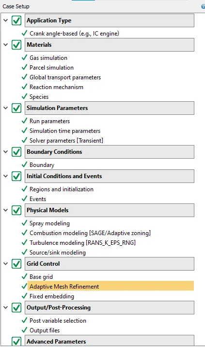
Application Type- Crank angle-based IC engine.

Gas simulation with along with Parcel simulation and Air as predefined mixture.

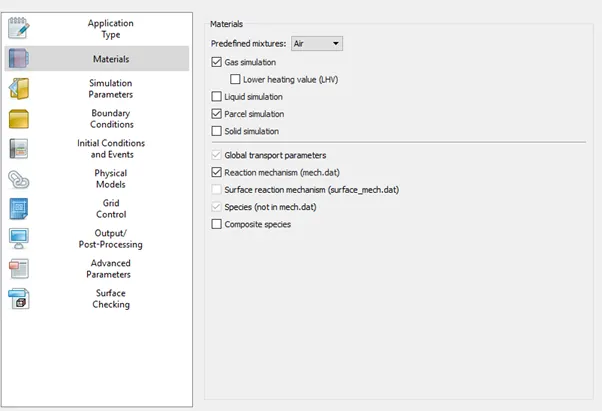
IC8H18 is selected from predefined liquid in Parcel simulation.

Density Based Transient State Solver is used with Compressible Gas Flow solver and Incompressible liquid Flow solver with no hydrodynamic simulation and PISO Navier-Stokes’s solver scheme.

The solution run for -480 deg to 240 deg which is 720 deg cycle.

Regions –

Cylinder Region:

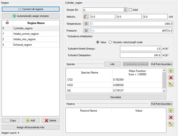
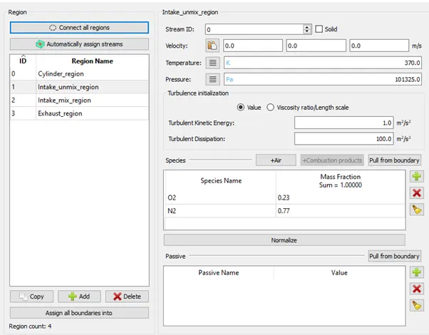
Intake_unmix_region:

Intake_mix_region:

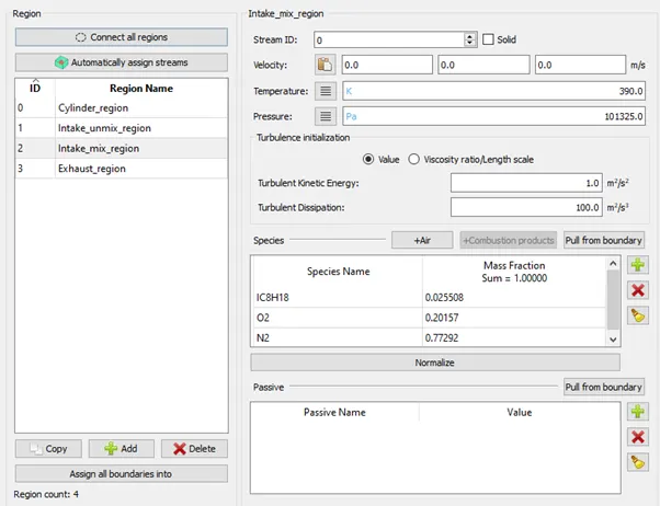
Exhaust_region:

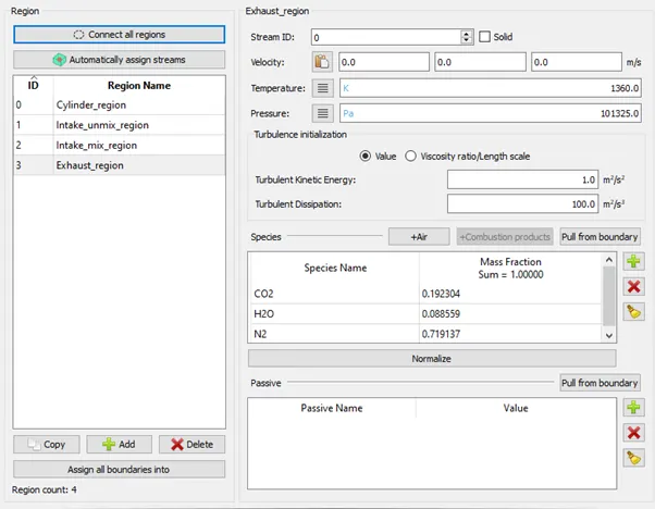
Regional group –

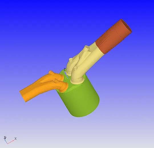
Boundary Condition:

Boundary	Region	Boundary Condition/ Motion	Temp (K)	Species
Inlet	Intake_unmix_region	Inflow	363 K	O2: 0.23 N2: 77
Intake_port_Unmix		wall Stationary	425 K
Intake_port_mix	Intake_mix_region	wall Stationary	425 K	IC8H18: 0.025508 O2: 0.20157 N2:0.77292
Inlet_valve_top		wall Translating	480 K
Inlet_valve_angle		wall Translating	480 K
Inlet_valve_bottom	Cylinder_region	wall Translating	480 K	CO2: 0.1932 H2O: 0.088525 N2:0.71913
Spark_plug		wall Stationary	550 K
Spark_plug_terminal		wall Stationary	600 K
Head		wall Stationary	450 K
Liner		wall Stationary	450 K
Piston		wall Piston Motion	450 K
Exhaust_valve_bottom		wall Translating	525 K
Exhaust_valve_angle	Exhaust_region	wall Translating	525 K
Exhaust_valve_top		wall Translating	525 K
Exhaust_port		wall Translating	500 K
Outlet		Outflow	800 K

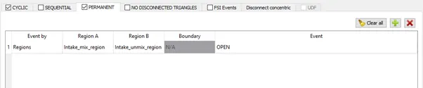
Event is marked in initial condition and events tab.

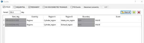
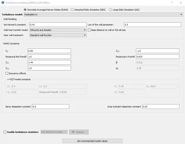
Realizable K-epsilon is used for turbulence modelling with recommended values.

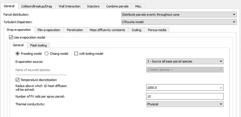
Spray Modeling is turned On. Colision mesh is checked and O'Rourke film spash model is used for wall Interaction. Solid cone spray injection type is used in which fuel is uniformly distributed throught the cone.

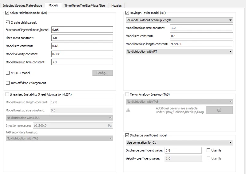
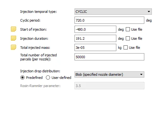
A injector is added with four nozzle with IC8H18 as fuel and KH along with RT model is used for Inector spray.

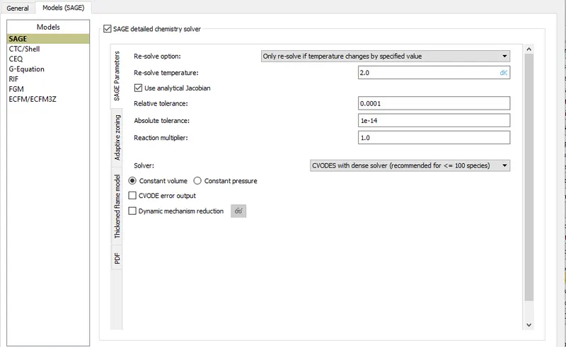
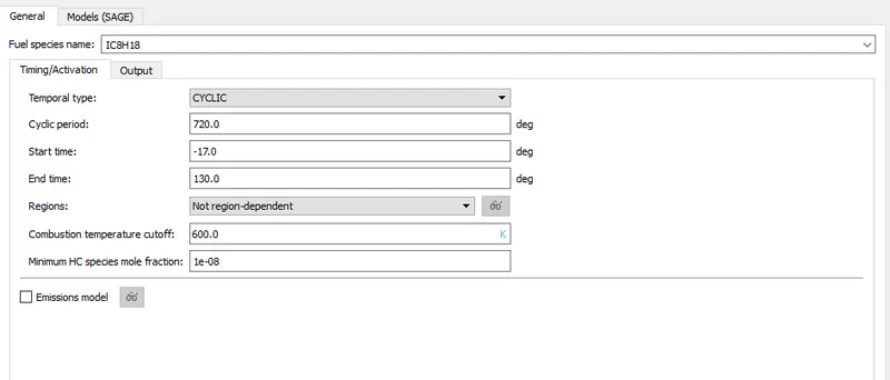
SAGE is used for Combustion Modelling.Adpative Zoning is used with bin temp 5 K.

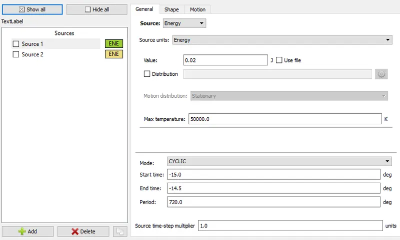
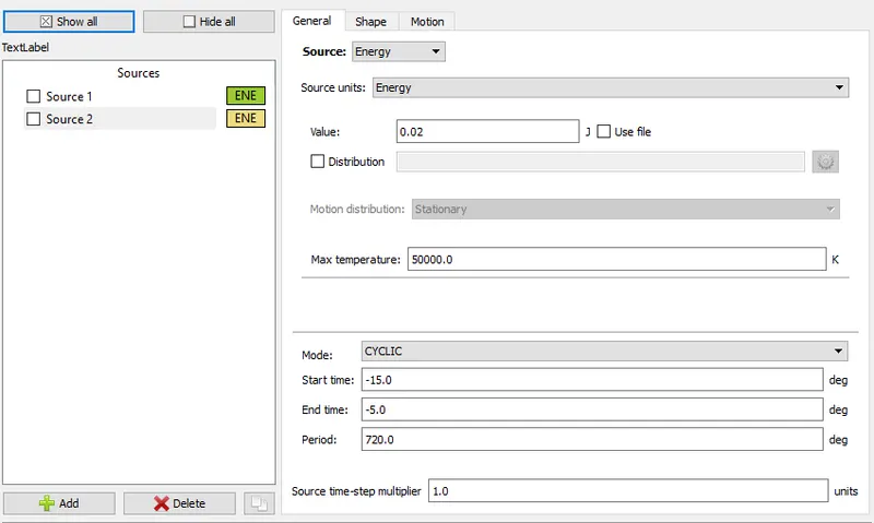
Source and Sink is also used to provide Spark Ignition in the Spark_plug.

Base grids of 0.005 m or other for respective cases are generated for all axis.

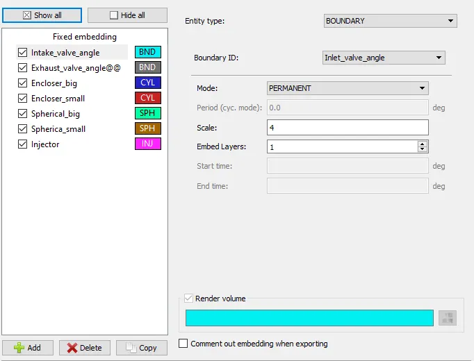
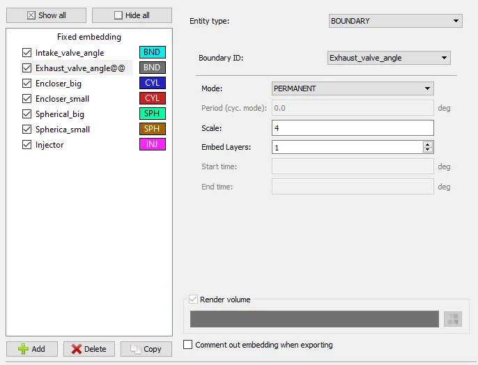
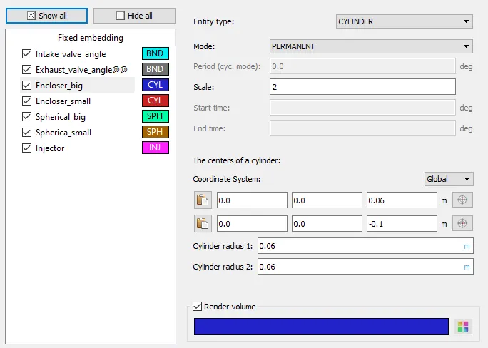
Fixed Embedding is marked in grid control tab and 7 embedding are added.

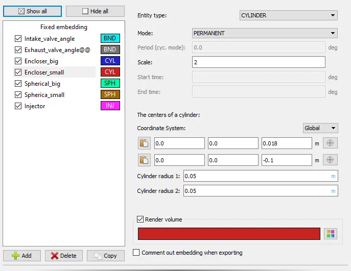
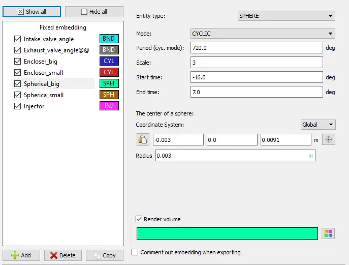
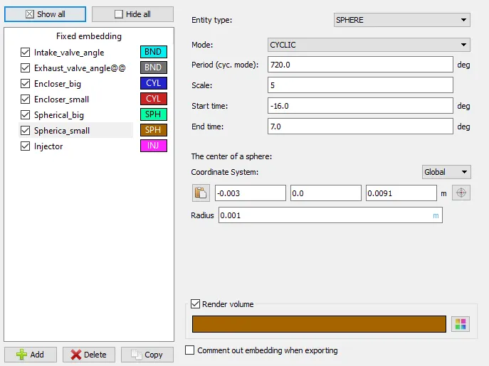
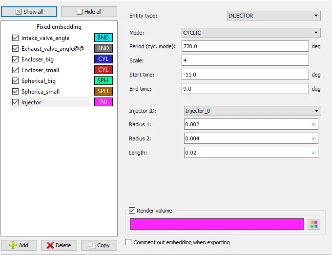
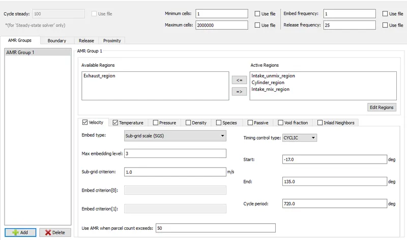
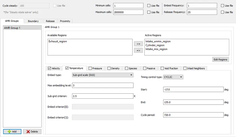
Adaptive Mesh Refinement is also used to refine Velocity and Temperature.

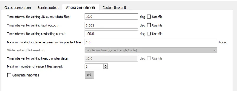
3D output data is written after every 10 deg.

The input files are exported to a folder to further solving.

Solving using Cygwin:

The Cygwin directory is navigated to the above saved folder and following code is entered to solve the problem.

mpiexec.exe -n 2 "C:\Program Files\Convergent_Science\CONVERGE\3.0.16\bin\intelmpi\converge.exe" restricted </dev/null> logfile &

where address in quotes gives the path of folder containing input file exported earlier.

Results:

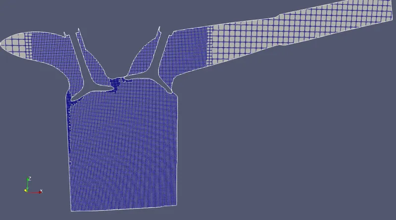
Initial Mesh –

Mesh Animation -

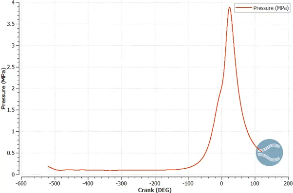
Pressure -

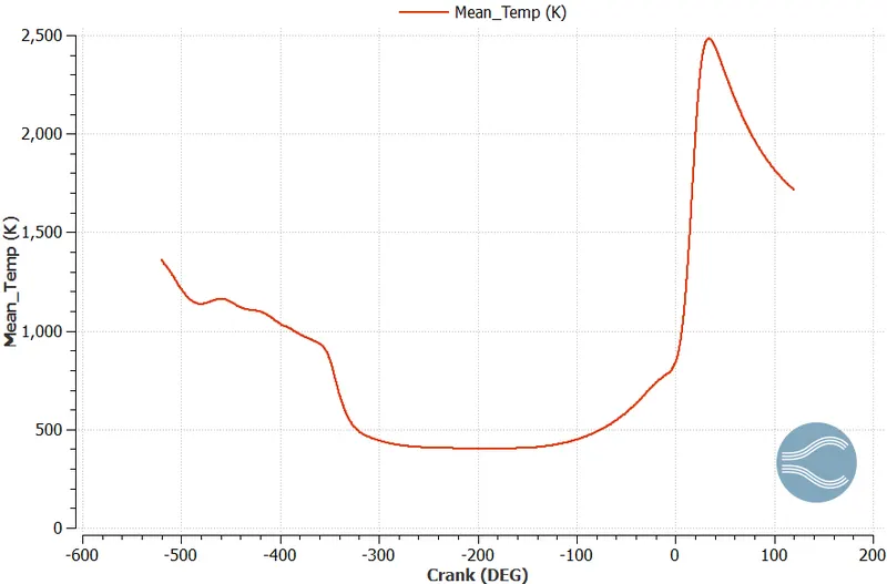
Temperature -

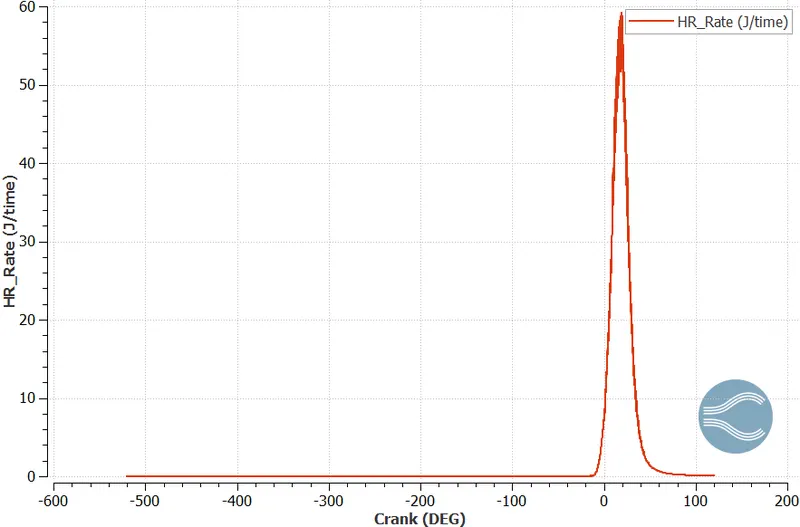
Heat Release Rate -

Compression Ratio - The compression ratio is the ratio between the volume of the cylinder and combustion chamber in an internal combustion engine at their maximum and minimum values.

`CR = (V_(swept) + V_(cl earence))/ V_(cl earence)

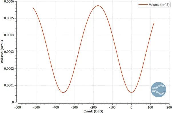
Here Vs + Vc = .000574 `m^3` & Vc = 5.75e-5 `m^3` at crank-angle 180 deg and 0 deg., Hence

CR = 9.892

Combustion Efficiency - It is defined as the ratio between the energy released by the burnt fuel and the theoretical energy content of the fuel mass during one complete engine cycle.

`eta_c = "Total Heat Released" / "Total Energy contentof fuel" = Q / (m_f * LHV)`

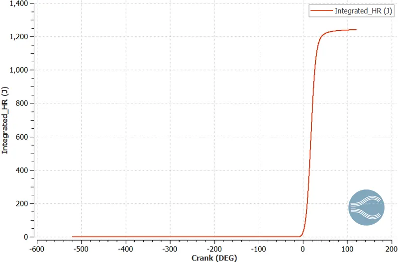
Here Q = 1241.1646 J from above graph. `m_f = 3e-5 kg` and LHV = 44.4 MJ/Kg

`eta_c = 1241.146 / ((3e-5) * (44.4e-6)) = 93.18 %`

Engine Performance -

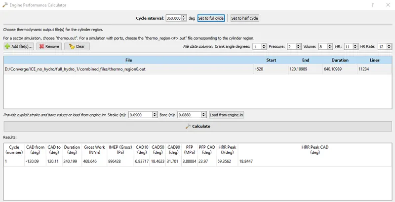
RPM	3000
RPS	3000/60 = 50
Degree /sec	50*360 = 18000
Duration (in deg.)	242.199 deg
time for work done	242.199/18000 = 0.01345 sec

Power = Gross Work / Total time = 468.646/ 0.01345 = 34.843 KW

`"Torque" = P/(2*pi*N)`

T = 34.843/(2*3.14*50) = 110.9 N-m

Significance of ca10, ca50 and ca90 -

'ca' stands for crank angle and values 10 50 and 90 represents the various percentage for which combustion happens at various crank angles.

• ca10 implies 10 % combustion at 6.83717 crank angle
• ca50 implies 10 % combustion at 18.4623 crank angle
• ca90 implies 10 % combustion at 31.701 crank angle

Need of Wall Heat Transfer Model -

In order to accurately predict Heat Transfer through wall heat transfer model is used, Since heat is important factor which impact efficiency and performance of the engine. A correct estimtion of wall heat flux can give better results. As thermal Boundary layer is very small and capturing the layer can provide accurate result but the size of the cell should be very small and hence requires time and calculation capacity. To avoide this heat transfer model is used which predicts heat flux transfer from fluid to solid/wall boundary interace as well as wall temperature.

CFD simulation do not accurately predicts the wall temperature as these sove NS equations and while Case setup the transport equation and are set for fluid domains. Similarly other valuse are set for the fluid regions while for solid- fluid interface and solid boundary condition are needed to accurately solve the heat equations.

CHT (Conjugate Heat Transfer) is used to solve both for fluid flows and Heat transfer together.

Spray Animation -