Week 10: Project 1 - FULL HYDRO case set up (PFI)
Introduction:
After post-processing, No-Hydro setup, & verifying the case parameters run as specified, 2nd part of this project have full hydrodynamic simulation including the combustion & spray modelling.
Objective:
- Modelling of the PFI engine.
- To run a fulll hydro simulation.
- Spray modelling & nozzle setup for the simulation.
Theory:
Spray Modeling:
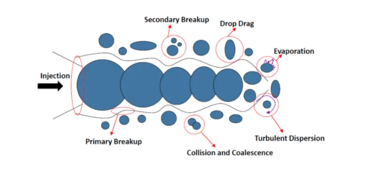
Converge uses state of art models for spray processes involving liquid atomization, drop breakup, collision & coalescence, turbulent dispersion & drop evaporation in terms of liquid sprays. Converge uses a Lagrangian solver to model discrete particles and Eulerian solver to model the continuous fluid domain. Lagrangian specification of the flow field is a way of looking at fluid motion where the observer follows an individual fluid parcel as it moves through space and time. Plotting the position of an individual parcel through time gives the pathline of the parcel. The Eulerian specification of the flow field is a way of looking at the fluid motion that focusses on specific locations in the space through which the fluid flows as time passes. The eulerian cell center is fixed while the lagrangian parcels move. Heat, momentum & mass transfer occur between the discrete and continuous phases via source terms in transport equations.
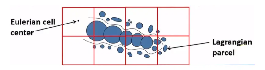
Parcels are introduced into the domain at the injector, which presents a group of identical drops with the same radius, velocity, and temperature. The parcel is the basic unit converge solves instead of drop. Parcel undergoes several physical processeslike a primary breakup, secondary breakup, drop, drag, collision & coalescence, and evaporation.
Evaporation Model:
The spray evaporation that takes place needs to be considered and for that converge uses certain standard pre-created models such as Frossling, Chiang, or with boiling. In this project, the Frossling model is used and it does not need to provide the particular equations as Converge takes care of it. Converge asks for evaporation source to simulate multi-component vaporization. The source used in this project is "Source all base parcel species" which denotes multi-component liquid species evaporate into the base species.
As the evaporation source is specified, the maximum radius of ODE droplet heating needs to be specified as well, its basically a temperature discretization parameter which will control if drop temperature is uniform or radially varying. If the drop radius exceeds maximum value the converge assumes a radially varying temperature or else uniform temperature distribution is assumed.
Spray Penetration and Distribution:
Converge writes the liquid and vapor penetration lengths at each output interval, it calculates vapor penetration length for each nozzle. For each cell that meets the criteria that fuel vapor mass fraction exceeds the user-specified value or cell size does not exceed user-specified bin size, converge calculates the center of the nozzle to the center of the cell.
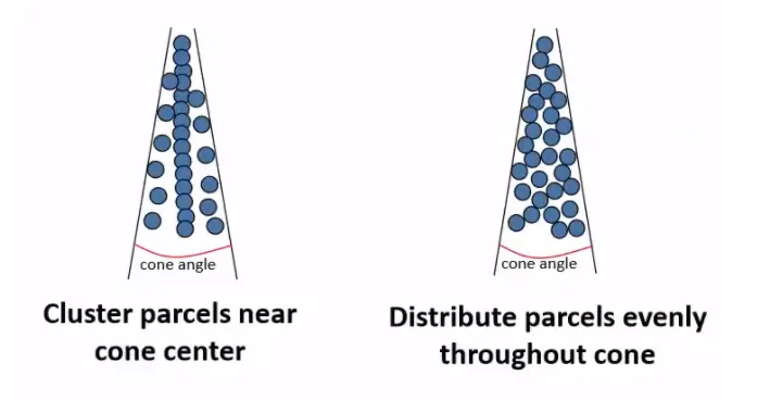
The parcel distribution is done in two ways where the parcels are either distributed evenly throughout the cone or clustered near the center of the cone. Depending upon the requirement either distribution can be selected, for this project, even distribution is selected.
Set up:
- This set up is different from the Part-1. Here, full hydrodynamic simulation is performed.
- For the Physical setup, the following models are selected. (Spray, Combustion, Turbulence, Source models)
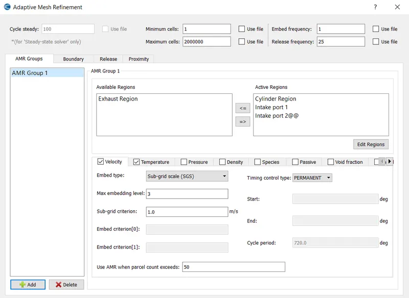
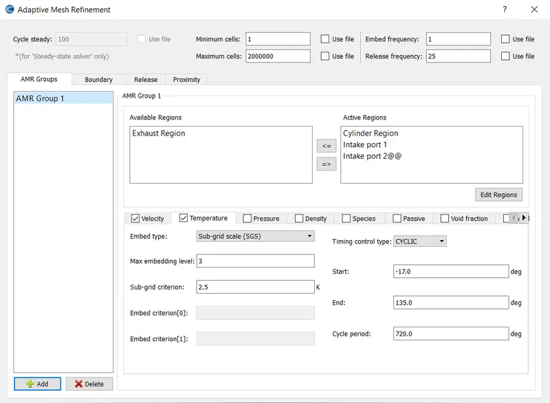
- AMR and embedding are incorporated in the Grid control section.
1. Engine Parameters
Bore : 0.086 m
Stroke: 0.09 m
Connecting Rod Length: 0.18 m
RPM: 3000
2. Regions and Initialization:
(A) Region 0 - cylinder:
Pressure: 1.85731 bar
Temperature: 1360 K
(B) Region 1 - Intake-1
Pressure: 1 bar
Temperature: 390 k
(C) Region 2 - Intake-2
Pressure: 1 bar
Temperature: 370 k
(D) Region 3 - Exhaust
Pressure: 1.85731 bar
Temperature: 1360 K
3. Boundary Conditions
(A) Piston
Boundary Type: Wall
Wall Motion Type: Translating -> Piston Motion
Wall Temperature: 450K
Region: Cylinder
(B) Liner and Cylinder Head
Boundary Type: Wall
Wall Motion Type: Stationary
Wall Temperature: 450K
Region: Cylinder
(C) Spark Plug
Boundary Type: Wall
Wall Motion Type: Stationary
Wall Temperature: 550K
Region: Cylinder
(D) Spark Plug Electrode
Boundary Type: Wall
Wall Motion Type: Stationary
Wall Temperature: 600K
Region: Cylinder
(E) Intake Ports 1 & 2
Boundary Type: Wall
Wall Motion Type: Stationary
Wall Temperature: 425K
Region: Intake-1 & Intake-2 respectively
(F) Exhaust Port
Boundary Type: Wall
Wall Motion Type: Stationary
Wall Temperature: 500K
Region: Exhaust
(G) Inflow
Boundary Type: Inflow
Pressure: 1 bar
Temperature: 363 k
Species: Air
Region: Intake-2
(H) Outflow
Boundary Type: Outflow
Pressure: 1 bar
Backflow Temperature: 800 k
Species: Stoichiometric composition (See Region 0)
Region: Exhaust
(I) Intake Valve Angle and Top
Boundary Type: Wall
Wall Motion Type: Translating -> intake_lift.in
Wall Temperature: 480 K
Region: Intake-1
(J) Intake valve Bottom
Boundary Type: Wall
Wall Motion Type: Translating -> intake_lift.in
Wall Temperature: 480 K
Region: Cylinder
(K) Exhaust valve Angle and Top
Boundary Type: Wall
Wall Motion Type: Translating ->exhaust_lift.in
Wall Temperature: 525 K
Region: Exhaust
(L) Exhaust Valve Bottom
Boundary Type: Wall
Wall Motion Type: Translating ->exhaust_lift.in
Wall Temperature: 525 K
Region: Cylinder
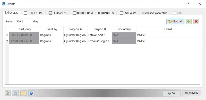
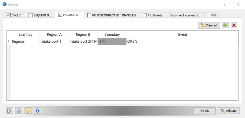
Events:
AMR:
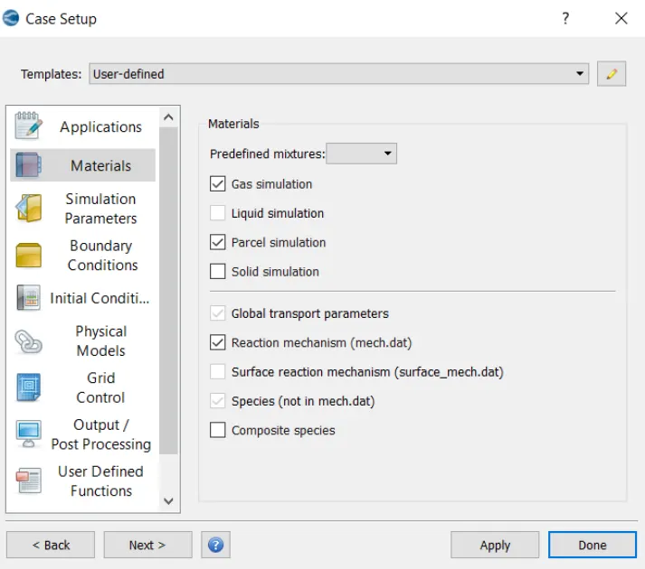
Parcel Simulation:
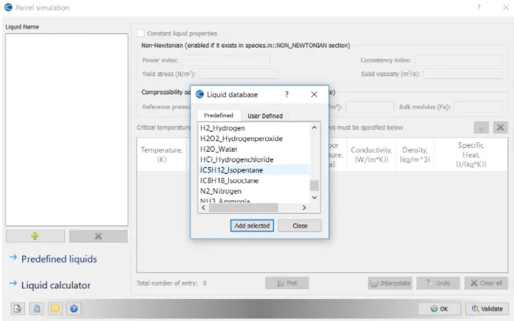
Injection Parameters:
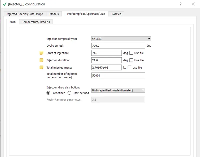
- Fuel flow rate = 7.5e-4 Kg/second
- Injection start time = -480.0
- Injection duration = 191.2
- Fuel temperature = 330K
| Fuel Flow rate (kg/s) | 7.50E-04 |
| RPM | 3000 |
| RPS | 50 |
| DPS(degrees/s) | 18000 |
| Time per degree | 5055556E-05 |
| Time per cycle(720 degree) | .04 |
| Fuel injected per cycle (kg) | 3.00E-05 |
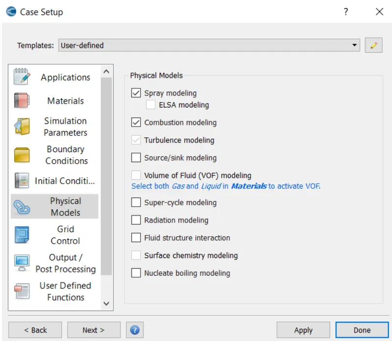
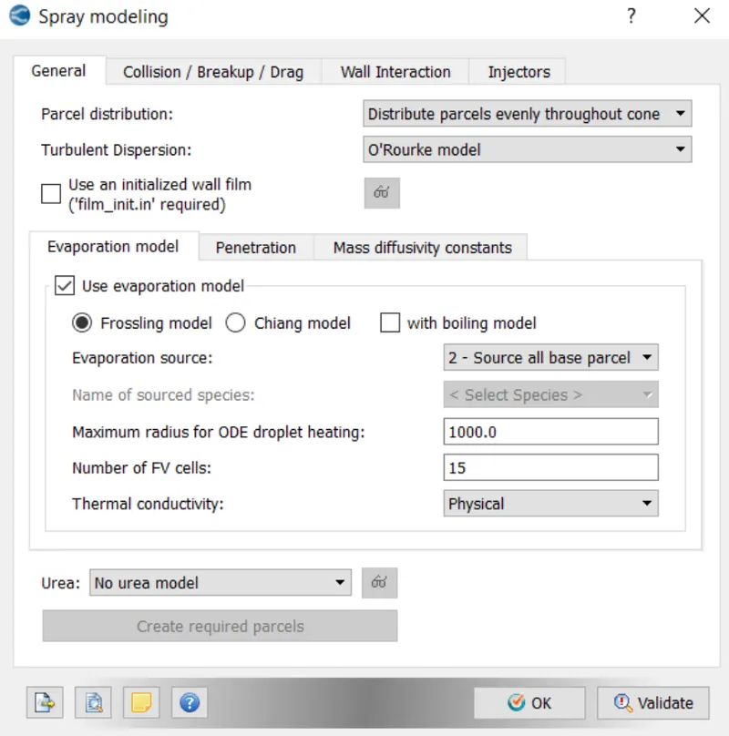
Respective models and recommended evaporation parameters are set.
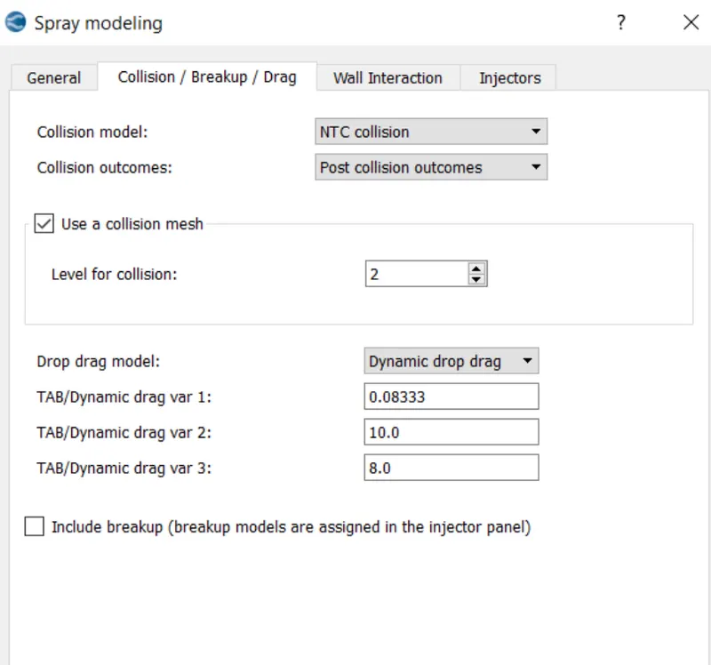
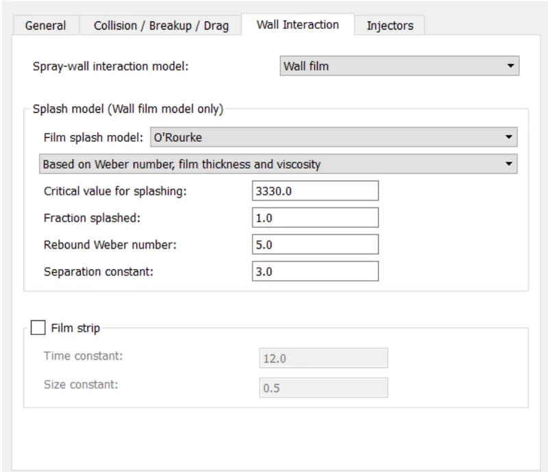
Collision mesh & modelling develop detailed meshes to count for the minor changes in aftermath of parcel to parcel Collison or onto the walls of the intake chamber.
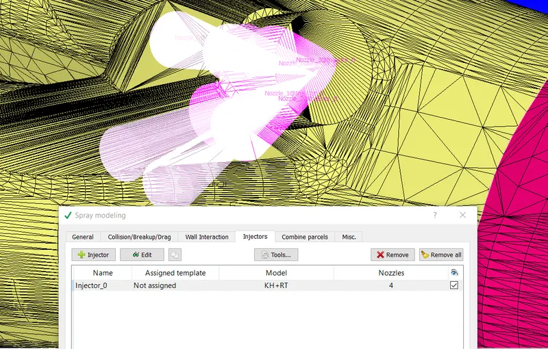
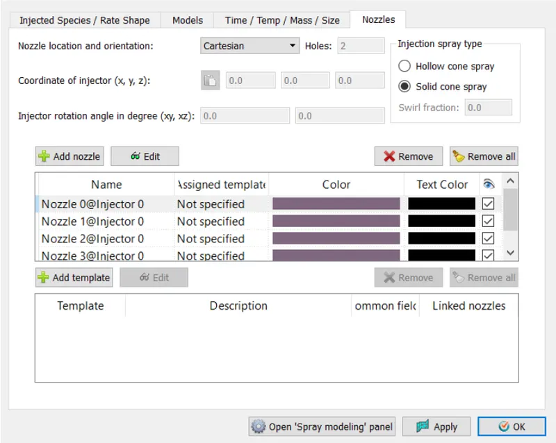
To incorporate 4 nozzles & designate respective alignment & cone angles for each of the nozzles.
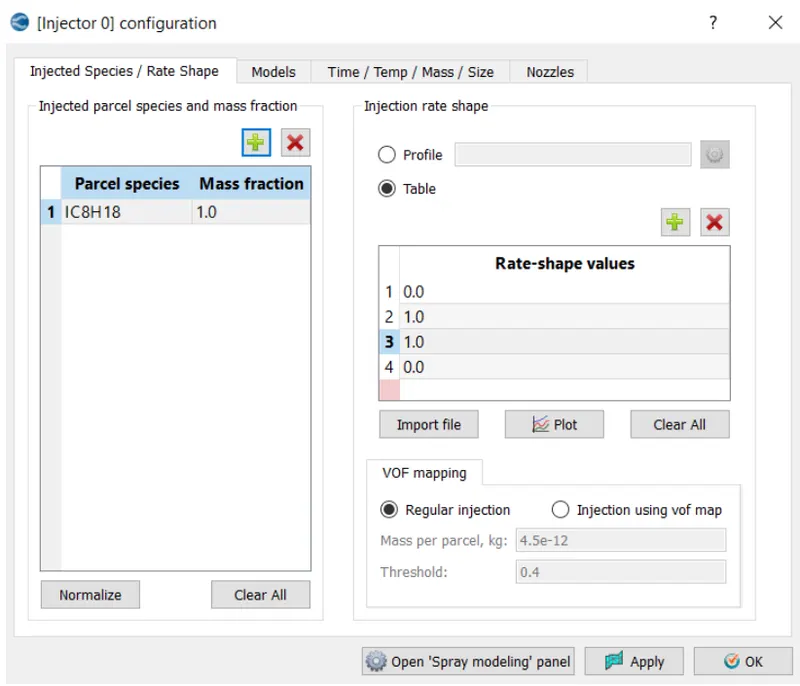
Select edit Injector dialog box to input the following characteristics:
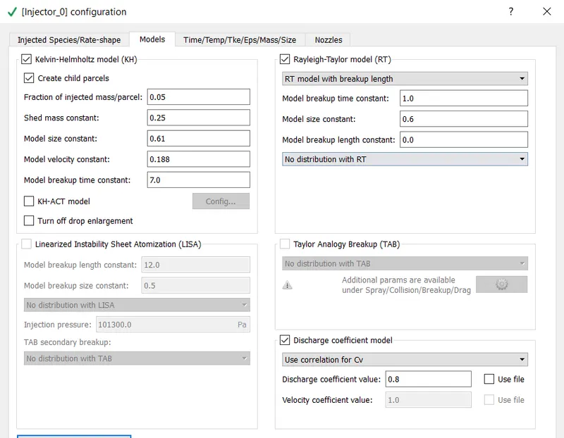
- Inject species - IC8H18 with the shape trapezoidal (0,1,1,0)
- KH and RT models with discharge coefficient 0.8
- Circular injection radius of each nozzle = Nozzle diameter/2.
The pressure at which nozzle functions can be calculated by using the tools.
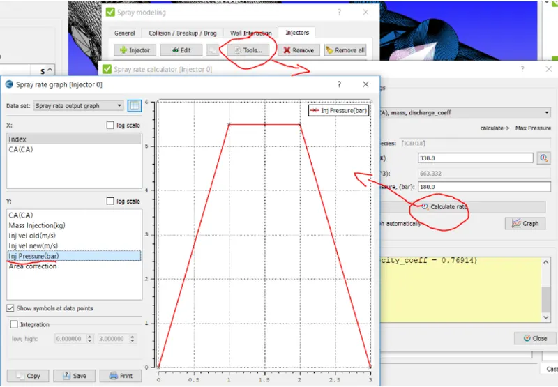
For a diesel engine, the pressure would be so high, in thousands of bars, because atomizing the diesel fuel is difficult and needs to be done at high pressure.
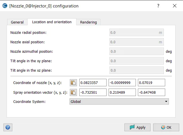
Nozzle Positions
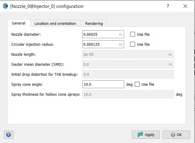
Nozzle diameter = 250 micro-meter
Circular injection radius = Nozzle radius
Spray cone angle = 10
- Nozzle 0
center 0.0823357 0.00100001 0.07019
Align Vector -0.732501 0.210489 -0.647408
- Nozzle 1
center 0.0823357 -0.00099999 0.07019
Align Vector -0.732501 -0.210489 -0.647408
- Nozzle 2
center 0.0823357 -0.0004 0.07019
Align Vector -0.5 -0.2 -0.647408
- Nozzle 3
center 0.0823357 0.0003 0.07019
Align Vector -0.5 0.2 -0.647408
SPARK SETUP
We need to input concentrated energy packets or source definition at specific intervals of time, right at the compression stroke for optimum combustion. For this, source/sink modeling is used.
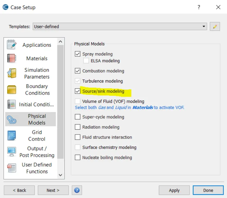
Through experiments, it has been found out that for the first 0.5 degrees along the combustion stroke to take place, we need to cross the dielectric barrier of air using 40 MJ of energy to initiate the spark & after that energy subsidies, a 20 MJ is maintained for smooth combustion.
Spark Ignition Parameter
- Start of spark = -15 deg
- Spark duration = 10 deg
- Spark location = -0.003 0 0.0091
- Spark radius = 0.0005m
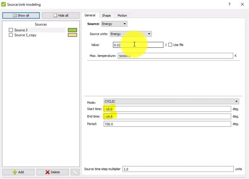
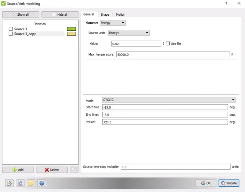
Two energy sources are given, with one having an added 0.02 J along with another 0.02 J across a duration of 10 degrees so that they add up to 0.04 J just in the interval of -15 to -5 degrees assigned to just one of the sources. This allows for a constant 0.02 J across the whole 10-degree duration.
Combustion Modelling:
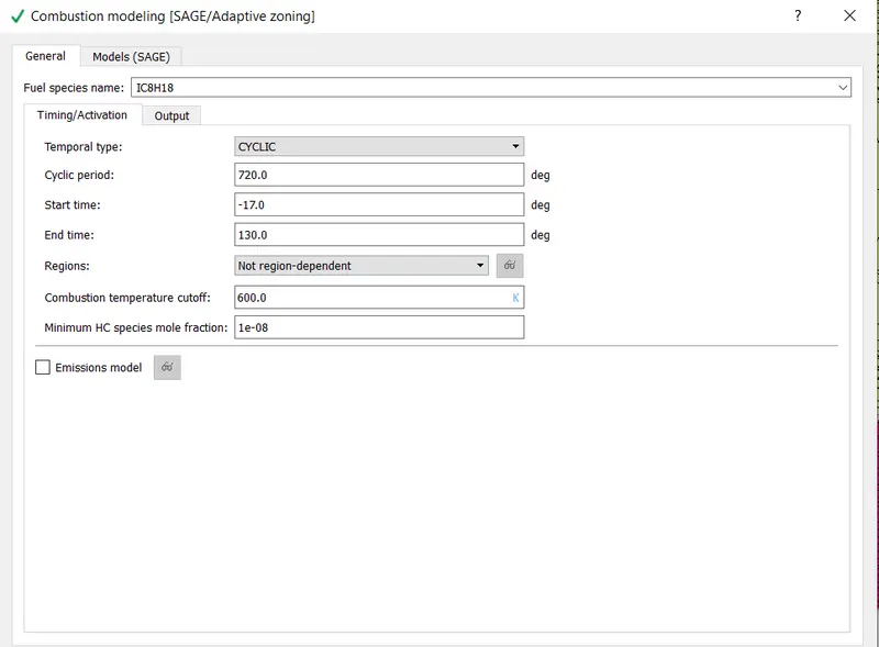
Combustion facilitates the energy transfer in the engine. Converge contains detailed chemistry solver and simplified combustion models. In the present project, we will be using SAGE detailed chemical kinetics solver.
SAGE:
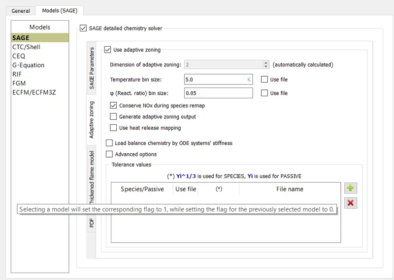
The SAGE detailed chemistry solver is a general combustion model used to solve the detailed chemical kinetics in the combustion process. It can accurately model ignition and laminar flame propagation. It uses local conditions to calculate reaction rates based on the principles of chemical kinetics. Also, determines kinetically limited phenomenon of engine knock and emissions. It requires a CHEMKIN-formatted input fils to solve the reaction rate ODEs. The ODE solver used is called as CVODE solver. SAGE couples with transport solver via source terms in the species transport equations.
The recommended combustion models are provided along with a multizone value for faster combustion. The end time is determined by the degree to which the exhaust valve opens.
Embedding
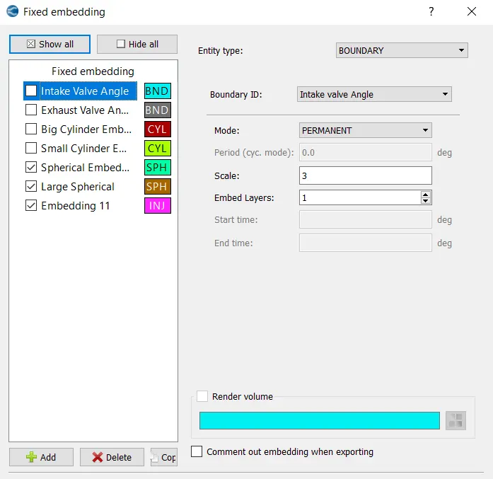
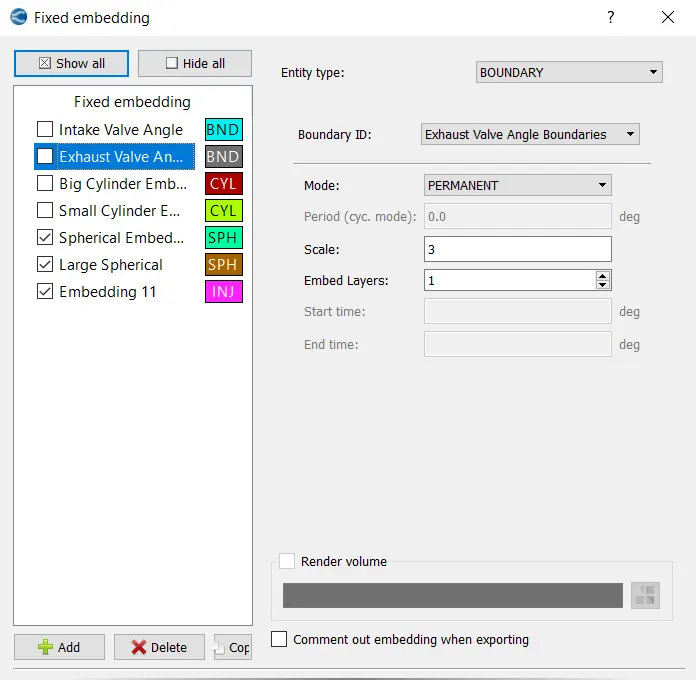
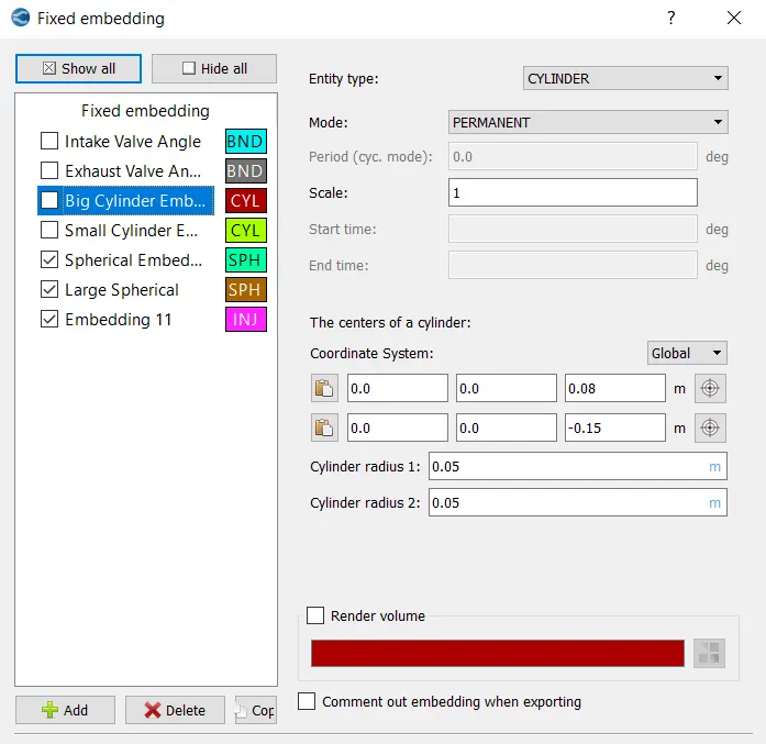
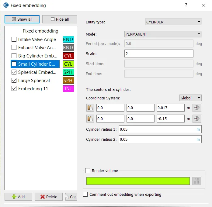
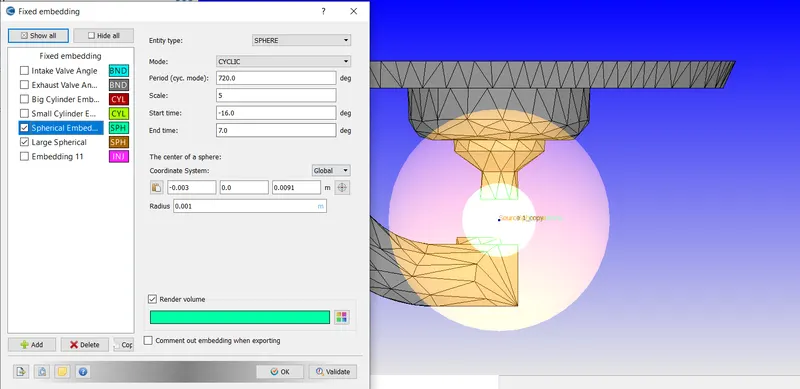
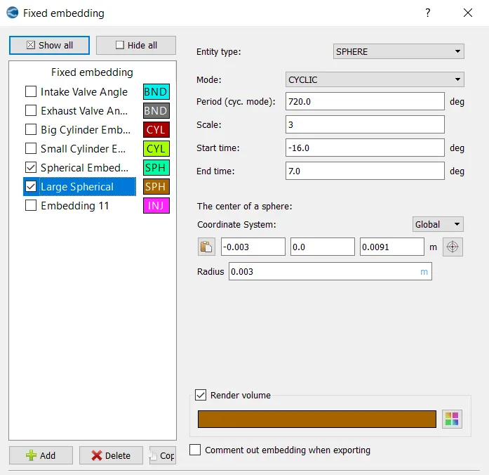
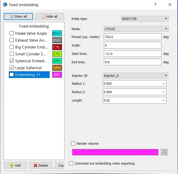
The larger sphere embedded for spark has been set as the scale of 3 & the smaller one is set as a scale of 5 for maximum gradient converge of temperature difference during ignition of fuel & combustion process.
Fuel Mass Calculation:
Given that the mass flow rate of fuel is 7.5e-4 kg/s and RPM of 3000, it is possible to calculate mass flowing per cycle for a period of 720 [deg].
RPM is converted to RPS which is further converted to DPS . From DPS we can determine the time taken for 720 [deg] and the mass flow in Kg can be obtained.
3000 RPM = 3000/60 RPS = 50 RPS
50 RPS = 50*360 DPS = 18000 DPS
Time taken for rotation by one degree is 1/18000.
Time per degree = 1/18000 DPS = 5.55e-5 s.
Time for 720 degrees = 5.55e-5 * 720 = 0.04s
So, the total mass of fuel injected per cycle is 7.5e-4 [kg/s] * 0.04 [s] = 3e-5 kg
PLOTS
Volume Plot
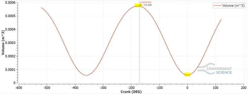
This plot defines the maximum and minimum volumes inside the cylinder during the whole simulation time period. A very important engine quantity can hence be derived using the plot itself, Compression Ratio
Compression Ratio
Compression ratio (CR) is defined as the action between the max. & min. volume in the cylinder.
Calculation:
Max. volume = 0.00057 m^3
in. volume = 5.7 x 10^-5 m^3
Hence, CR = Max.vol/Min.vol = 0.00057/5.7 x 10^5 = 10
Hence, the Compression ratio of the engine is 10:1
Pressure Plot
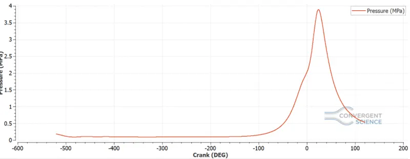
The pressure plot shows that peak pressure is achieved during the compression stroke, followed by the combustion stroke. After release of kinetic energy due to combustion, the pressure drops to its normal value as seen in the plot.
Heat transfer rate plots
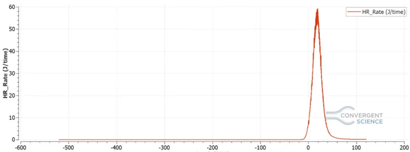
Trap mass plot
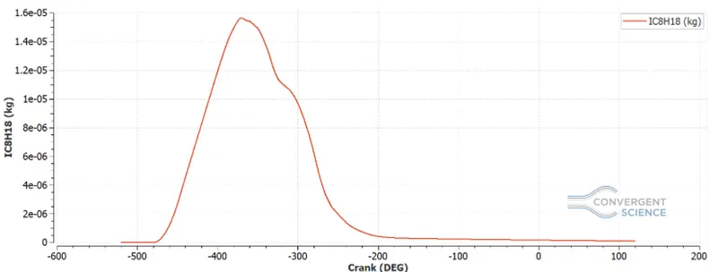
The trap mass is the mass of fuel present around the intake valve portion and intake port itself, not taking part in the combustion process.
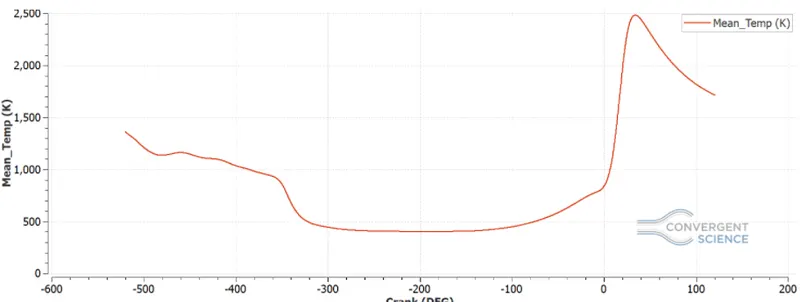
Temperature plot
Integrated HR Plot
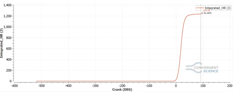
The integrated heat transfer is the net amount of energy released in the engine. In this case, the max value of 1241 J is the output energy we get from the combustion process. Using this, we can calculate the combustion efficiency of the engine by incorporating the mass & low heating coefficient of the fuel with the integrated heat transfer. From this, we can get the amount of input energy given in the form of fuel & the amount of energy we got as output from the engine.
Combustion efficiency
Combustion efficiency is the ratio between output energy derived from the engine to input energy provided to the engine. It determines how efficiently the combustion process has occurred in the engine.
Calculation:
Energy Output = 1241 J
Mass of fuel/cycle used = 3 x 10^-5 kg
Lower heating value of fuel used, C8H18(isooctane) = 3 x 44.8 x 10^-5 x 10^6 = 1344 J
Hence, Efficiency = Output/Input = 1241/1344 = 92.33%
The combustion efficency of the engine is 92.33%
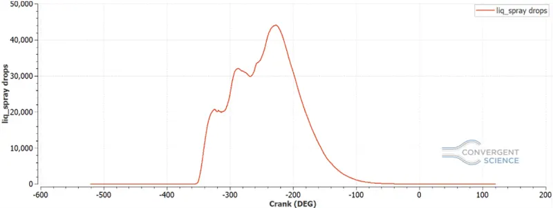
Spray Parcel plot
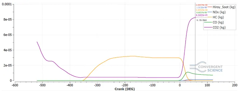
Emission Plot
Q. Why do we need a wall heat transfer model? Why can't we predict the wall temperature from the CFD simulation?
Ans. ->
The entire PFI engine simulation takes place a long time to run since it includes several physical phenomena interacting with each other that is fluid flow, turbulence, injection, ignition, combustion, etc. Also, for the simulation, only the fluid domain is modelled & the outer walls of the cylinder it intake and exhaust ports are not modeled. Due to the complex physical interaction taking place inside the regions & the absence of physical properties for the walls, it is not ideal to calculate the wall temperatures based on CFD alone.
Engine Performance Calculator
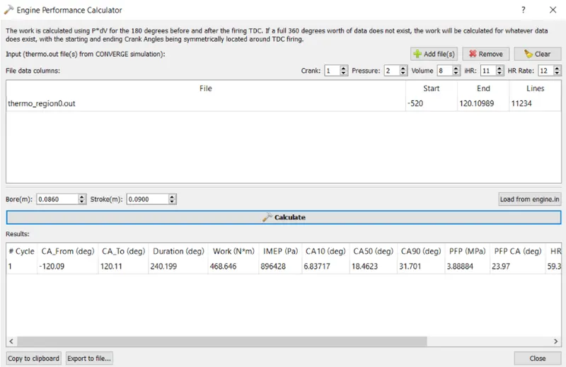
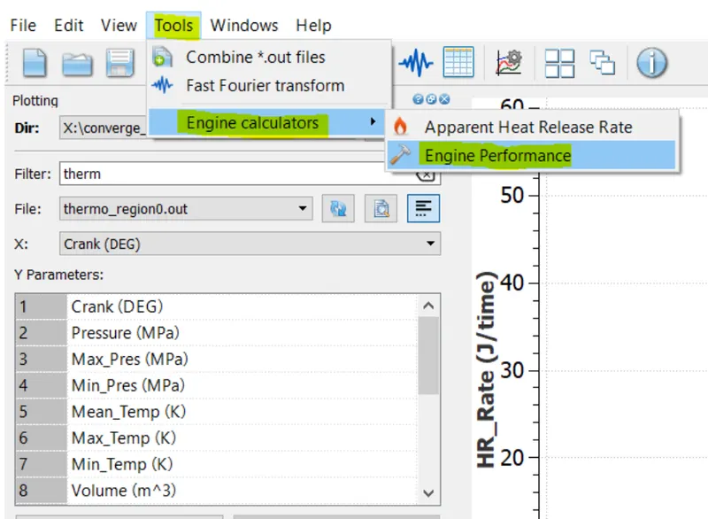
The engine performance calculator is used to analyze physical data & get results from the data simulated. We can find the calculator from the line plot models in CONVERGE CFD, tools tab.
We have to load a set of data such as:
Duration of combustion = 240.19 degrees
Work done = 468.646 N-m
IMEP (Indicated Mean Effective Pressure) = 8.96 Bar
CA10 = 6.83
CA50 = 18.46
CA90 = 3.17
Power is nothing but the amount of work done per unit time.
where Time is the time of combustion
Power = work/Time
Calculation:
We know that work done = 468.646 Nm.
Time of combustion = 240.199
Revolutions per minute = 3000
Revolutions per second = 3000/60 = 50
Degrees per second = 50 x 360 = 18000
Time of combustion = (240.199/18000) = 0.0133 s
Power P = Work /Time = 468.646/0.0133 = 35.236.54 J/s = 35.236 kW
We also know that, Power(P) = (2*pi*N*T)/60
Hence, Torque = 111.78 Nm
What is the significance of CA10, CA50, AND CA90?
CA10, CA50, and CA90 defined as the crank angles of 10%, 50%, and 90% of the max accumulated apparent heat release.The crank angle at which 10%, 50% and 90% of the combustion have been completed respectively. The significance of these values is that engineers can use this as a reference to reduce the time taken or crank angle at which most of the combustion takes place, as unburnt fuel is a waste of energy & also produce black soot that adds to the tailpipe exhaust pollution.
Simulation Link:
Combustion Simulation:
https://drive.google.com/file/d/1Xgtm4KxiCofpm1ET4sQl5ofquChLd23h/view?usp=share_link
Flame Propogation:
https://drive.google.com/file/d/1A4KvdY8O6_zKTQWv6tsPH_HuBEjhrgtB/view?usp=share_link
Conclusion:
Thus, simulation of PFI engine is done.