Port Fuel Injection combustion simulation using O'Rouke Model.
Objective: To simulate the Full-hydro case setup of PFI.
1. Explain the compression ratio definition and calculate the same for the given engine.
2. Calculate the Combustion efficiency of the Engine.
3. Determine the Power and torque of the engine by using an engine performance calculator.
4. Explain the significance of CA10, CA50, and CA90.
5. Evaluate the need for a wall heat transfer model. Why can't directly predict wall temperature from CFD simulation?
Given:
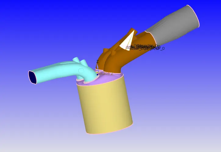
The parameters which are necessarily required to run a complete full hydrodynamic simulation of PFI are given below:
1. Engine Geometric Parameter
2. Run Parameters
3. Simulation time parameter
4. Boundary condition
5. Initial condition
6. Injection parameter
7. Nozzle Position
8. Spark Ignition parameters.
Introduction
The gasoline port fuel injection is the most popular drive system for gasoline engines worldwide. The powertrain system convinces with low costs, reduced technology, and new, innovative further developments.
The expected motion of the Engine :
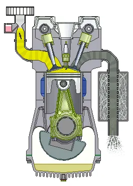
an internal combustion (IC) engine in which the piston completes four separate strokes while turning the crankshaft. A stroke refers to the full travel of the piston along the cylinder, in either direction. The four separate strokes are termed:
Intake: Also known as induction or suction. This stroke of the piston begins at the top dead center (T.D.C.) and ends at the bottom dead center (B.D.C.). In this stroke, the intake valve must be in the open position while the piston pulls an air-fuel mixture into the cylinder by producing vacuum pressure into the cylinder through its downward motion. The piston is moving down as air is being sucked in by the downward motion against the piston.
Compression: This stroke begins at B.D.C, or just at the end of the suction stroke, and ends at T.D.C. In this stroke, the piston compresses the air-fuel mixture in preparation for ignition during the power stroke (below). Both the intake and exhaust valves are closed during this stage.
Combustion: Also known as power or ignition. This is the start of the second revolution of the four-stroke cycle. At this point, the crankshaft has completed a full 360-degree revolution. While the piston is at T.D.C. (the end of the compression stroke) the compressed air-fuel mixture is ignited by a spark plug (in a gasoline engine) or by heat generated by high compression (diesel engines), forcefully returning the piston to B.D.C. This stroke produces mechanical work from the engine to turn the crankshaft.
Exhaust: Also known as an outlet. During the exhaust stroke, the piston, once again, returns from B.D.C. to T.D.C. while the exhaust valve is open. This action expels the spent air-fuel mixture through the exhaust valve.
When using engines with specific performance of approx. 60 kW/l and downsizing concepts of up to 25%, the gasoline port fuel injection offers significant cost advantages compared with high-pressure direct injection systems. As a low-pressure system (system pressure approx. 6 bar), the gasoline port fuel injection operates with a comparatively simple operating strategy. The complex high-pressure control requirements (system pressure up to 350 bar) are omitted as are the high-pressure pump, the high-pressure sensor, the volume control valve, and the high-pressure injectors for multi-point injections. The result is a less complex injection control using variances regarding the injection time frame. The robust combustion process of the gasoline port fuel injection also tolerates fuel of lower quality.
In this project, CFD simulation for the PFI engine system is developed with spray modeling, combustion modeling, and full hydro setup for extracting results for critical engine parameters responsible for judging engine performance.
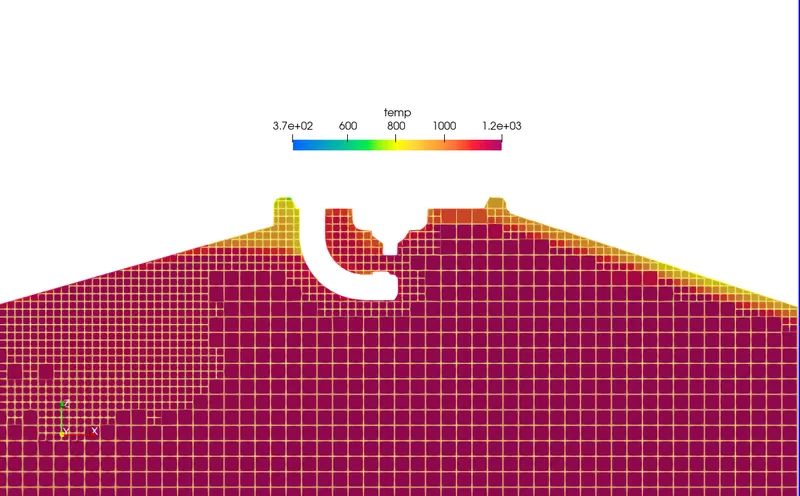
The analysis is done at the operating point i.e. 3000 rpm and full load condition. The parameters are kept constant throughout the study both physical and chemical. AMR refinement was utilized with velocity and temperature SGS criterion. Fixed embedding was also utilized to influence and enhance the accuracy of AMR.
Case set up for Full Hydro Simulation :
Design Parameters
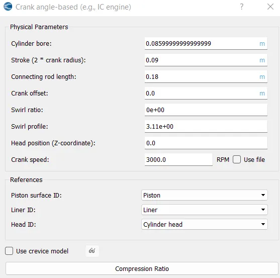
The application type is set to Crank angle based as we are simulating an IC engine cylinder.
The measurements for the cylinder are specified by referring to the given data file.
Cylinder Bore : 0.086 m
Stroke: 0.09 m
Connecting rod length : 0.18 m
Crank speed: 3000 RPM
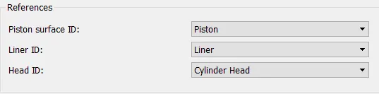
Specify the reference boundaries as given below, so that the motion of the simulations takes place at the right boundaries.
Import the mech.dat and therm.dat in the tree of the material to specify the reactions taking place between the materials inside the cylinder during combustion.
In the run parameters, set up a transient simulation and select Hydrodynamic solver as simulation mode. The gas flow solver is set to be compressible.
The simulation time parameter is set from -520 degrees to 120 degrees as the simulation is made to run for a total of 720-degree angles.
Materials:
In IC engine simulation focus will be more interested in knowing reactions inside the combustion chamber after combustion takes place, how the fuel will be injected inside the cylinder during suction/ Intake stroke of the engine, what will be participating species or what will be the type of fuel we are going to inject inside the cylinder. This will be done in this Materials section by selecting the proper type of fuel and respective parameters.
IC8H18 (Iso-Octane)- It has physical properties that are closer to the physical properties of GASOLINE fuel. That is the reason we chose Parcel species as "IC8H18".
Since we have selected IC8H18 as parcel species we will require its thermodynamic data to involve more species in the reaction mechanism contained in the file named "therm.dat".
Boundary Conditions
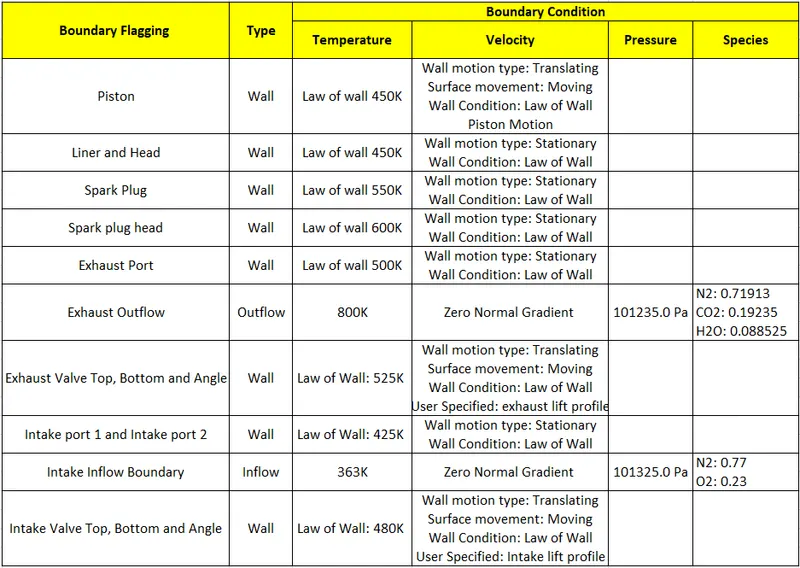
The intake and exhaust valves have three differently named walls. This is done to assign walls to proper regions and also the connection of two regions is dependent on this naming. The valve bottom walls are walls of the cylinder region. To restrict the flow during the closed position of valves, the cylinder and manifold regions need to be physically separated. In the real world, the seals in valve seats prevent the flow between these regions but this can't be done during simulations because the geometry would intersect and cause an error in simulation. To overcome this, the software creates a virtual interface wall between regions that are to be disconnected. The valve angles are the walls whose boundary edges will be used when the software would create the virtual interface.
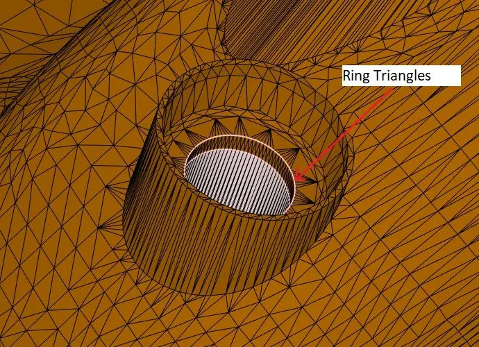
The valves will move along their stem axis. When this happens, the valve bottom, angle, and stem move together and intersection errors are cleared but, the surface to which the stem is joined, also moves. This is prevented by using ring triangles when the stem moves, the ring triangles stretch along the stem axis. Thus preventing the deformation of the top surface.
The exhaust valve top, bottom, and angle are taken as moving walls following the profile of a given data file (Exhaust_lift.in).
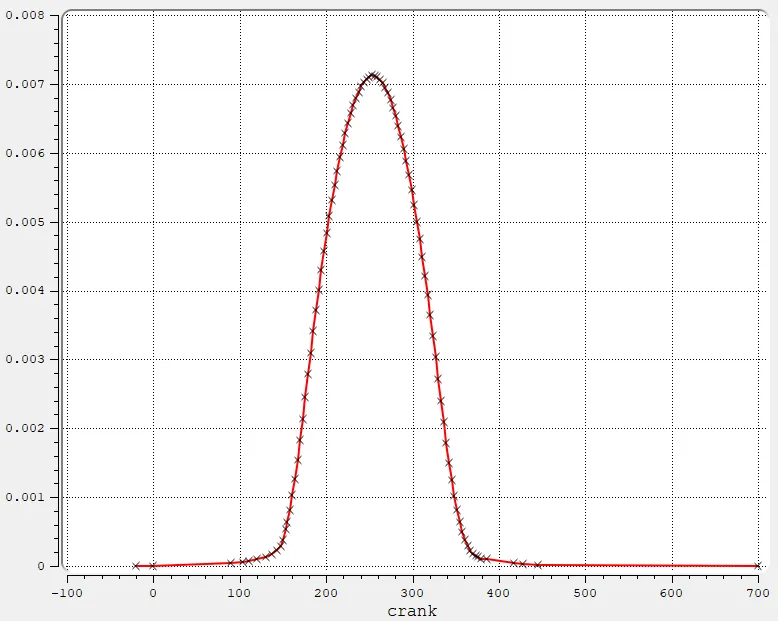
TEMPORAL
valve
direction  0.27537 0 -0.96134
min_lift  2.e-4
CYCLIC         720.0
crank          lift
-20.0          0.0
0.0            0.0
89.5710        4.27061e-05
103.400        5.91945e-05
111.09         7.56830e-05
120.0          0.0001
130.816        0.000136907
137.520        0.000177117
143.445        0.000228068
147.895        0.000292514
150.234        0.000370760
153.249        0.000534956
154.59         0.00063274
157.67         0.00081932
160.74         0.0010317
163.82         0.0012697
166.89         0.0015335
169.97         0.0018295
173.04         0.0021383
176.12         0.0024536
179.19         0.0027817
182.27         0.003097
185.34         0.0034123
188.42         0.0037147
191.5          0.0040106
194.57         0.0042937
197.65         0.0045704
200.72         0.0048278
203.8          0.0050787
206.87         0.0053103
209.95         0.0055355
213.02         0.0057414
216.1          0.0059344
219.17         0.0061146
222.25         0.0062819
225.32         0.0064298
228.4          0.0065714
231.47         0.0066872
234.55         0.0067966
237.62         0.0068867
240.7          0.0069639
243.77         0.0070283
246.85         0.0070732
249.93         0.0071055
253.0          0.0071247
256.07         0.0071183
259.15         0.007099
262.23         0.0070604
265.3          0.0070089
268.38         0.0069382
271.45         0.0068609
274.53         0.0067645
277.6          0.0066486
280.68         0.0065264
283.75         0.0063848
286.83         0.0062239
289.9          0.0060567
292.98         0.0058765
296.05         0.005677
299.13         0.0054647
302.2          0.0052395
305.28         0.0050015
308.36         0.0047505
311.43         0.0044932
314.5          0.0042165
317.58         0.0039334
320.66         0.0036439
323.73         0.0033415
326.81         0.0030326
329.88         0.0027174
332.96         0.0024021
336.03         0.0020868
339.11         0.0017844
342.18         0.0015013
345.26         0.0012504
348.33         0.0010188
351.41         0.00081932
354.48         0.00064561
357.56         0.00049763
360.63         0.00038181
363.71         0.00029174
366.79         0.00022096
369.86         0.00017592
372.94         0.00014375
376.01         0.00012445
379.0          0.00010578
386.0          0.0001
417.024        4.93255e-5
428.092        3.16101e-5
444.862        1.49867e-5
700.0          0.0
Similarly, the inlet valve top, bottom, and angle are also taken as moving walls following the profile of a given data file (Inlet_lift.in).
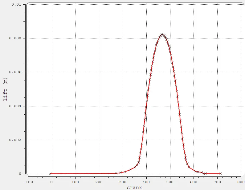
TEMPORAL
valve
direction  -0.309018 0 -0.951056
min_lift  2.e-4
CYCLIC         720.0
crank          lift
-6.0           0.0
272.248        2.35488e-05
290.107        5.56690e-5
309.30         0.0001
332.895        0.000232081
351.715        0.000379550
361.573        0.000521791
367.287        0.000664032
368.59         0.00072974
371.67         0.00094492
374.74         0.0011898
377.82         0.0014644
380.89         0.0017686
383.97         0.0021099
387.04         0.0024661
390.12         0.0028297
393.19         0.0032082
396.27         0.0035718
399.34         0.0039353
402.42         0.0042841
405.5          0.0046254
408.57         0.0049519
411.64         0.005271
414.72         0.0055678
417.8          0.0058572
420.87         0.0061244
423.95         0.0063841
427.02         0.0066215
430.1          0.0068441
433.17         0.0070519
436.25         0.0072449
439.32         0.0074155
442.4          0.0075788
445.47         0.0077123
448.55         0.0078385
451.62         0.0079424
454.7          0.0080314
457.77         0.0081057
460.85         0.0081575
463.93         0.0081947
467.0          0.0082169
470.07         0.0082095
473.15         0.0081872
476.23         0.0081427
479.3          0.0080833
482.38         0.0080018
485.45         0.0079127
488.53         0.0078014
491.6          0.0076678
494.68         0.0075268
497.75         0.0073636
500.83         0.0071781
503.9          0.0069851
506.98         0.0067774
510.05         0.0065473
513.13         0.0063025
516.2          0.0060427
519.28         0.0057682
522.36         0.0054788
525.43         0.005182
528.5          0.0048629
531.58         0.0045364
534.66         0.0042025
537.73         0.0038537
540.81         0.0034975
543.88         0.003134
546.96         0.0027704
550.03         0.0024068
553.11         0.002058
556.18         0.0017315
559.26         0.0014421
562.33         0.001175
565.41         0.00094492
567.271        0.000797031
572.879        0.000577014
580.456        0.000375818
607.793        0.000149310
619.50         0.0001
633.937        7.99912e-5
643.280        3.8451e-06
650.0          0.0
714.0          0.0
A minimum lift of 0.2 mm is given to get the required cell dimension to capture the gap by refinement. Increasing this gap would result in an inaccurate solution and reducing this value lesser would also increase the computational time required.
Initial Condition and Events:
Region and Initialisation:
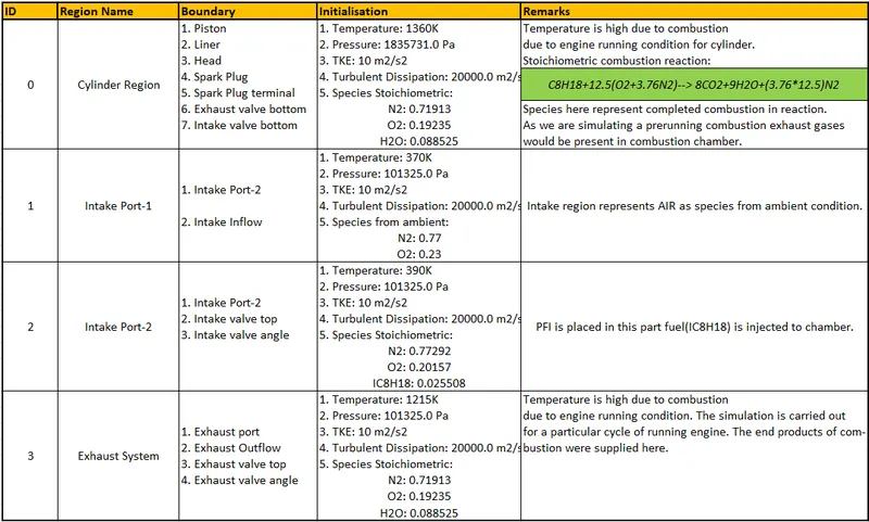
Events:
For two regions to be in contact with each other with no boundary between them, it is necessary to use events. The events create triangles in place between them, known as disconnect triangles. Events can be a permanent, cycle, or sequential. The disconnected triangles are imaginary triangles that are created by converge and are not visible in geometry. These are temporary and disappear after a given sequence/time period of simulation of an event. There should be no intersection in Converge geometry, therefore, the need for the events appeared to create a mechanism of interaction between two regions.
From the Events, dialog box creates custom CLOSE (activate disconnect triangles), OPEN (deactivate disconnect triangles), or VALVE events between two or more regions at defined intervals. Because CONVERGE cannot properly execute a simulation if surface triangles from two boundaries intersect, using the Events section is the only way to discontinue (or allow) flow between two regions.
Note: If we select a VALVE event, you must include a valve profile file.
That's why both the intake and exhaust lift profiles are provided.
Opening and closing of Intake and Exhaust valves play a key role in the IC engine. To simulate valves events are useful which are created as:
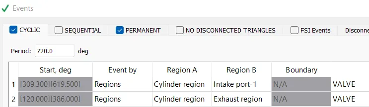
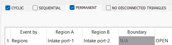
Turbulence & Physics modeling :
The first step in physics modeling is to set up the injection of fuel into the cylinder at a specific interval of time. Largest turbulent length scales in IC engine range from 0.1 to 1mm. During combustion turbulence stretches the flame surface area on which reactions occur, causing faster burning and flame extinction due to overstretching of the flame surface.
In non-premixed engines, combustion depends on the rate of fuel-air mixing. Turbulence increases the rate of mixing. The turbulence model is used to capture small-length scales. For turbulence modeling, one can select from a host of both RANS and LES models. The k-epsilon model is utilized in this simulation to solve turbulence closure modeling.
Spray Modeling :
CONVERGE includes state-of-the-art physical models for a wide variety of phenomena, including chemistry, turbulence, multiphase fluid flow, spray, and radiation, and it automatically couples these models. For a shorter runtime, one of CONVERGE’s simplified combustion models could be chosen. If accuracy is paramount, CONVERGE’s detailed chemical kinetics solver would obtain the results needed. For spray modeling, CONVERGE can capture physical processes from liquid injection and spray breakup to drop/wall interaction and evaporation. CONVERGE also includes several volumes of fluid modeling options to simulate multi-phase flows.
Converge introduces parcels(collection of drops) into the domain at the injector. Each parcel represents a group of identical drops (i.e same radius, velocity, temperature, etc).
Converge solves for radius, and velocity on a per parcel basis rather than a per drop basis (because the drops in a parcel are identical). The parcels statistically represent the entire spray field. Parcels undergo several physical processes such as a primary break-up, drop drag, secondary break-up, collision and coalescence, turbulent dispersion, and evaporation.
For liquid sprays, converge uses a lagrangian solver to model discrete parcels and the eulerian solver to model continuous fluid domain.
Select the spray modeling parameter in the physics models. In the spray modeling, we are using the O'Rourke model to initialize the spray of fuel.
The species to be injected is selected as the fuel element IC8H18, which is selected as the parcel particle in the properties of the materials.
The following parameter values are introduced for the specifications of fuel injection.
Fuel flow rate = 7.5e-4 Kg/second
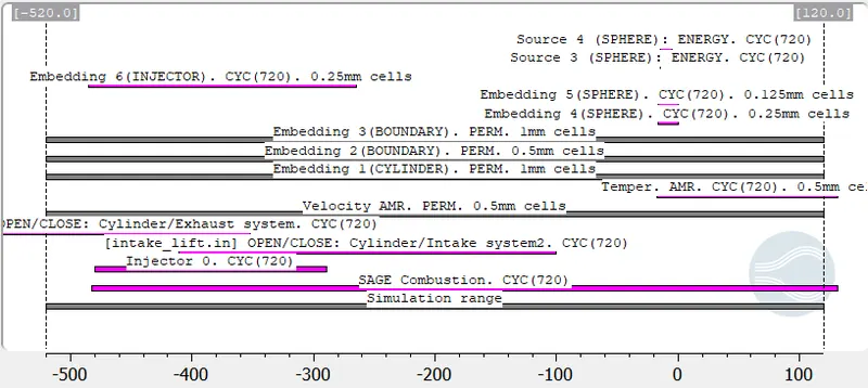
Injection start time = -480.0
Injection duration = 191.2
Fuel temperature = 330K
The rate shape profile was defined as trapezoidal. This profile will be used with shape, converge will take total mass values and total time, and it will automatically arrange those values in a trapezoidal profile.
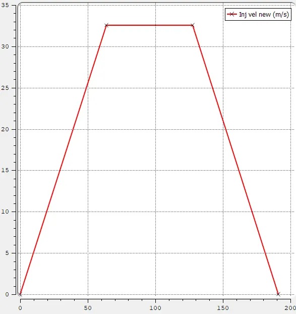
The Kelvin-Helmholtz (KH), Rayleigh-Taylor (RT) & Discharge coefficient models are being used for the injection.
Here, we are using four nozzles for spraying the fuel into the cylinder with similar specifications as follows.
Nozzle diameter = 250 micrometer
Circular injection radius = Nozzle radius
Spray cone angle = 10
To initialize this process, the Coordinates of the injectors are needed to decide the location at which the fuel is being emerged into the cylinder. The injectors will be located in the import region-1 which is located near the cylinder. The injector position and align vector is generally given by the design team.
Nozzle 0
center [0.0823357; 0.00100001; 0.07019]
Align Vector [-0.732501; 0.210489; -0.647408]
Nozzle 1
center [0.0823357; -0.00099999; 0.07019]
Align Vector [-0.732501; -0.210489; -0.647408]
Nozzle 2
center [0.0823357; -0.0004; 0.07019]
Align Vector [-0.5; -0.2; -0.647408]
Nozzle 3
center [0.0823357; 0.0003; 0.07019]
Align Vector [-0.5; 0.2; -0.647408]
Combustion Modeling
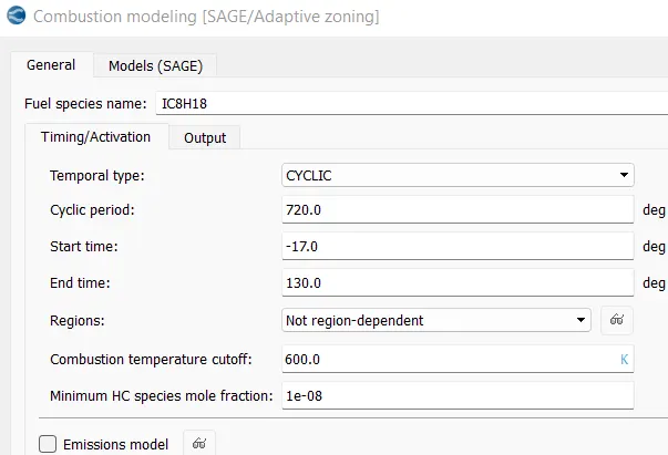
Converge's SAGE detailed chemistry solver uses local conditions to calculate reaction rates based on the principles of chemical kinetics. This solver is fully coupled to the flow solver, but the chemistry and flow solvers parallelize independently of one another, which speeds up the simulation. With the appropriate mechanism, the SAGE solver can predict a wide range of cases (e.g., a variety of fuels [premixed, non-premixed, partially premixed, multiple fuels], emissions modeling, and unique phenomena such as end-gas auto-ignition). With its accuracy and robustness, CONVERGE can perform predictive modeling instead of merely confirming experimental results. SAGE is three times slower than transport (species, momentum, turbulence equations) because we are solving at every cell and timestep.
SAGE: The species are modeled using chemical kinetics ODEs and the values are used in species transport equations. The Solver used to solve the ODEs is CVODES.
Acceleration technique: The SAGE solver is a detailed chemistry solver, meaning that it would calculate values based on the full mechanism instead of reducing it. This takes a lot of time if the calculations are done for every cell in the mesh. So, to increase the speed of solving, the solver is run using a multi-zone model. All the cells where combustion is going to be solved, are grouped into bins. The bins are created based on the temperature and equivalence ratio of fuel and air. All the cells having the same temperature and equivalence ratio will have the same combustion results. So, the SAGE solver is solved once for each bin, and accordingly, the flow and species data are remapped to the cells. This increases the speed tremendously. The bins can also be created based on multiple variables like pressure, reaction ratio, etc.
The multi-zone model reduces the number of SAGE calculations by grouping them into bins (zones). The number of bins varies dynamically with the stratification of the flow field parameters. Mapping the solved quantities to all cells in the bin, the bin is a kind of categorization. A single bin can have more cells.
Source Modeling
The spark plug is set up as an energy source. Source/sink modeling was enabled. Enable two sources for a given location.
In the source, modeling adds two sources where both the sources have a spherical shape.
Spark location = -0.003 0 0.0091
Spark radius = 0.0005m
| Source 1 | Source 2 | |
| Start time | `-15.0^@` | `-15.0^@` |
| End time | `-14.5^@` | `-5^@` |
| Value | 0.02J | 0.02J |
| Period | `720^@` | `720^@` |
| Mode | Cyclic | Cyclic |
The spark develops from the breakdown, arc, and glow stages. To approximately model this profile, 2 heat sources were utilized.
Meshing
Fixed Embedding:
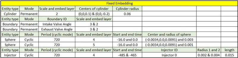
Depending on the flow dynamics, it was required that the flow in some regions was needed to be accurate and precise, while in some regions it could be more approximate. This can be done by varying the mesh element sizes in the region. The embedding option in Converge CFD does this work of creating finer mesh at the mentioned location. The refinement is based on scale and the number of embedded layers.
`dx_(embed) = (dx_(base))/(2^(embed_("scaling"))).`
`=4/(2^n)` for n=1,2,3,4,5
=2mm, 1mm, 0.5mm, 0.25mm and 0.125mm.
Adaptive Mesh Refinement:
The fixed embedding setting is preferred when the refinement is needed in the complete region or complete boundary area. When the refinement is to be done based on the solution of flow equations, the refinement technique is called AMR. The AMR monitors the solution and based on the curvature (second degree of rate of change) of a variable, the mesh is refined.
Advantages:
-
By eliminating the process of manual mesh creation, inspection and refinement, time is saved
-
Accuracy is improved through higher grid density where it is needed and where manual meshing strategies might not allocate it
-
AMR provides a robust method for capturing large or rapid boundary motions
-
AMR provides run-time savings due to using an optimized number of computational cells
-
Consistency and standardization can be achieved through the use of a consistent, algorithmic strategy for mesh production.
Adaptive mesh refinement is done to capture the places at which the properties of the calculation are critical.
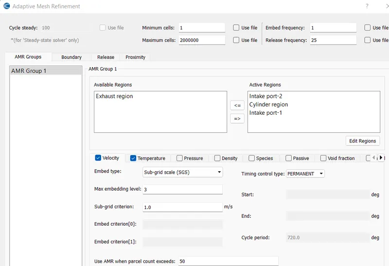
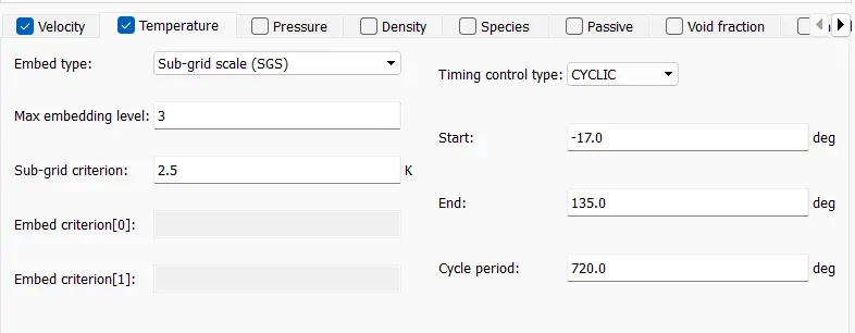
The refinement is made to be adaptive for velocity and temperature. If the grid was coarse, curvature values will also be lower and AMR will not properly mesh. Cell size can be calculated by turbulence length calculations.
The parameters for both properties are specified so that the mesh adapts the values from the specification to refine the places where the values tend to be within the specified parameter.
There are two methods to use AMR: The sub-grid scale method and the Value-based method.
In the value-based method, the value of the solution is specified. The mesh is refined if the value is more/less than specified.
A cell is embedded if the absolute value of the sub-grid field is above a user-specified value. Conversely, a cell is released (i.e., the embedding is removed) if the absolute value of the subgrid is below 1/5th of the user-specified value. That means if the user specifies a value of 2.5, the meshing program would calculate the sub-grid of the cell, based on the term shown above and if it is larger than 2.5, the cell will be refined.
|
Base grid |
dx, dy, dz : (0.004, 0.004, 0.004) m |
|
---------------------------------------------------------------------------------------------------------------------
Compression Ratio:
The compression ratio is the ratio between the volume of the cylinder and combustion chamber in an IC engine at their maximum and minimum values.
A fundamental specification for such engines, it is measured two ways: the static compression ratio, calculated based on the relative volumes of the combustion chamber and the cylinder when the piston is at the bottom of this stroke, and the volume of the combustion chamber when the piston is at the top of its stroke. In thermo.out plot volume vs crank angle in cylinder region.
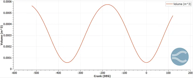
Compression ratio= `"Maximum value"/"Minimum value"`=`0.0005742195/(5.7539186e-5)`=9.98.
Combustion efficiency:
In practice, the exhaust gas of an IC engine contains incomplete combustion products (e.g., CO, H2, unburned hydrocarbons, soot) as well as complete combustion products (CO2, and H2O).
Under lean operating conditions the amounts of incomplete combustion products are small. Under fuel-rich operating conditions these amounts become more substantial since there is insufficient oxygen to complete combustion. Because a fraction of the fuel's chemical energy is not fully released inside the engine during the combustion process, it is useful to define a combustion efficiency.
The combustion efficiency ηc is defined as the ratio between the energy released by the burnt fuel and the theoretical energy content of the fuel mass during one complete engine cycle. `eta_c=(H_R-H_P)(T_A)/(m_f*Q_(HV))`
where:
HR [J] – enthalpy (internal energy) of the reactant
HP [J] – enthalpy (internal energy) of the product
TA [K] – ambient temperature
mf [kg] – a mass of fuel inducted per cycle
QHV [J/kg] – a heating value of the fuel
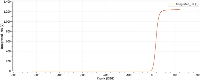
Integrated Heat Rate: It indicates the total amount of energy we are getting from the combustion process alone.
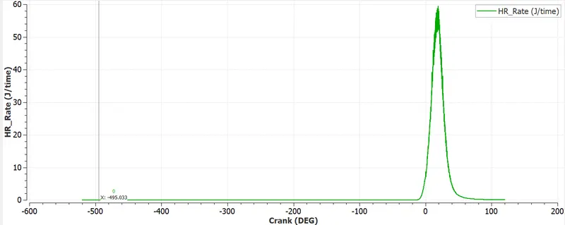
Combustion Efficiency calculated as:
From the graph,
Output power is 1240.72 J
Energy content of fuel= Mass of fuel inducted per cycle * Fuel LHV"> Mass of fuel inducted per cycle * Fuel LHVMass of fuel inducted per cycle * Fuel LHV
Where, Fuel Lower Heating Value (LHV) of ISOOCTANE is 44400 KJ/Kg
Mass inducted is `3E-5`.
`eta_c=1240.72/(444000*3E-5)`
The combustion efficiency will be found as,
Combustion efficiency `(eta_c)`=0.9315 or 93.15%.
Wall Heat transfer model:
The Heat loss through the walls of the engine is an important parameter during engine optimization, as it influences power, efficiency and emissions, and engine component thermo-mechanical reliability. As a consequence, a correct estimation of wall heat fluxes is mandatory. However, due to the complexity of the phenomenon involved in the heat transfer mechanism, such estimation is far from being trivial. Hence, accurate modeling techniques need to be available.
To predict the wall temperature by CFD simulation will require 10-15 cycles of engine which will take a lot of time for computation.
As we know this process of decomposition is called meshing. The bodies in the flow are often treated as "VOID" or "HOLES". The surface of the body becomes one of the boundaries of the computational domain and the appropriate boundary conditions must be set on it to obtain a numerical solution.
Determining Power and torque of engine by using an engine performance calculator:
To open performance calculator go to Line plotting in converge CFD.
Go to Tools --> Engine calculators --> Engine performance.
Give the thermo.out file for the cylinder region as the input file for calculating the engine's performance.
Import engine.in for engine geometrical data. Click on calculate.

Power = Work/sec
From performance calculator we can take;
Work = 486.646 Nm
Start time = -120.09 deg
End time = 120.11 deg
Total duration = 240.199 deg
Total rotation per minute RPM = 3000 (Given)
Rotation per second = 3000/60 = 50.
Total degree per second = 50*360 = 18000
Time in sec = 240.199/18000 = 0.01334 sec.
Power = 468.646/0.01334= 35130.88456W= 35.130KW
TORQUE
`P=(2*pi*N*T)/60`
P=Power
N=Rotation speed (rpm)= 3000rpm
T= Time
`T =(P*60)/ (2*pi*N)`
N = 3000 RPM.
`T = 35.130 *1000* 60 / (2*3.14*3000)=111.8789 N.s`
Significance of CA10, CA50 and CA90
The CA 10, 50, 90 here represent stages of combustion where 10, 50, 90% of total fuel mass is combusted respectively.
Mass Fraction Burn (MFB) is used to evaluate ignition delay and combustion duration by dividing the amount of accumulated fuel or accumulated heat during the combustion period by the total fuel or total heat release.
The combustion state occurring in the cylinder can be distinguished by MFB.
From the start of fuel injection, the crank position where MFB becomes 10% is noted as CF10, the point where MFB becomes 90% is noted as CA90.
CA50 denotes where the MFB is 50%, which means that 50% of injected fuel is converted into energy.
The difference between fuel injection point start and CA10 is called Flame-development Angle or Ignition Delay. And the Difference between CA10 and CA90 is called Rapid-burning Angle or Combustion Duration.
Time Map of simulation processes:
Plots of flow properties in the combustion chamber :
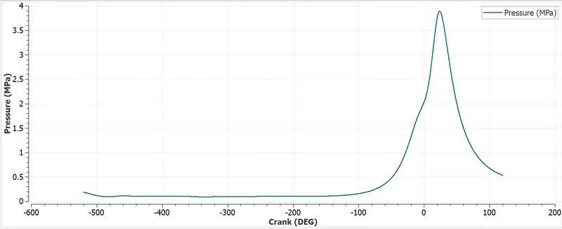
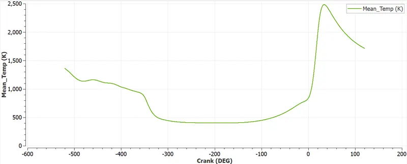
The mean temperature is maximum (2454.37 k) at the point when the integrated heat release is close to its max value, i.e. the entire heat energy is released. It is also the point where there is maximum pressure in cylinder (3.654 Mpa).
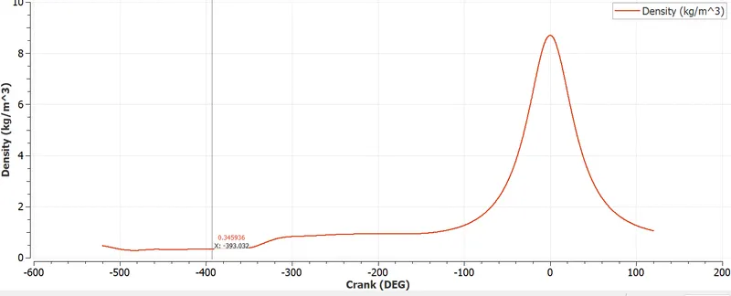
Total Cell Count:
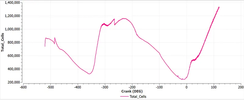
Maximum Total cells were 1328490 at crang angle of 119degrees.
Animation:
PARCEL:
The parcels increased as injection started. The parcels started collecting in films on cylinder wall when the intake valves were open. This is because when the intake valves were fully open, the fuel spray was directly hitting the cylinder wall.
Temperature
Here, visualization of flame propagation takes place inside the combustion chamber after initiating spark in the spark plug. Also, it can be seen how well AMR has performed inside the cylinder in order to capture the data at every crack angle.
The combustion chamber initially has a medium temperature as the exhaust stroke ends. The temperature in the exhaust port can be found to be maximum at the begining. This is because of the high temperature emission of the exhaust gases through the exhaust port.
The intake port has a minimum value as it sprays the fuel particles into the chamber. During expansion the temperature inside the chamber gradually decreases and attains a minimum value.
Once all the fuel particles enters the chamber the inlet valve closes and the piston moves up to compress the fuel. At this time the temperature is gradually increasing.
At the time of ignition there is a sudden increase in the temperature which spreads through out the chamber and the heat is transfered to the walls of the combustion chamber.
CONCLUSION:
- Engine efficiency was found to be 93%.
- All required calculations were done to find torue and power.
- Engine was run for 720degrees.
- Spraymodeling was utilised with cone angles and spray ejection position data.
- Neccesary animation and plots were processed to gather more ensights of engine critical parameters.