Week 10: Modeling and Simulation of flow around an Ahmed Body
Objective:
To simulate flow around an Ahmed body.
- Creating the CAD model using any CAD package
- Setup a Coarse CFD simulation
- Setup the virtual wind tunnel as shown in the video
- Apply the right boundary conditions and solver settings
- Use a coarse mesh to demonstrate that your setup runs successfully .
- You need to show an animation of the velocity distribution on a cutplane. This cutplane should cut the ahmed body model in two symmetric pieces.
- You need to show an animation of the pressure distribution on a cutplane. This cutplane should cut the ahmed body model in two symmetric pieces.
- Enable wall-averaged outputs to measure the drag and lift forces
- Calculate the steady state drag force value and explain your calculation procedure.
- Calculate the drag co-efficient using paraview and explain your calculation process in detail.
Ahmed body:
The Ahmed body is a geometric shape first proposed by Ahmed and Ram in the year 1989. the shape provides a model to study geometric effects on the wakes of ground vehicles.
Wake is a region of disturbed flow (often turbulent) downstream of a solid body moving thjrough a fluid , caused by the fluid around the body. It is a region of recirculating flow immediately behind a moving or stationary body, cvaused due to viscosity and may be accompanied by flow separation or turbulence.
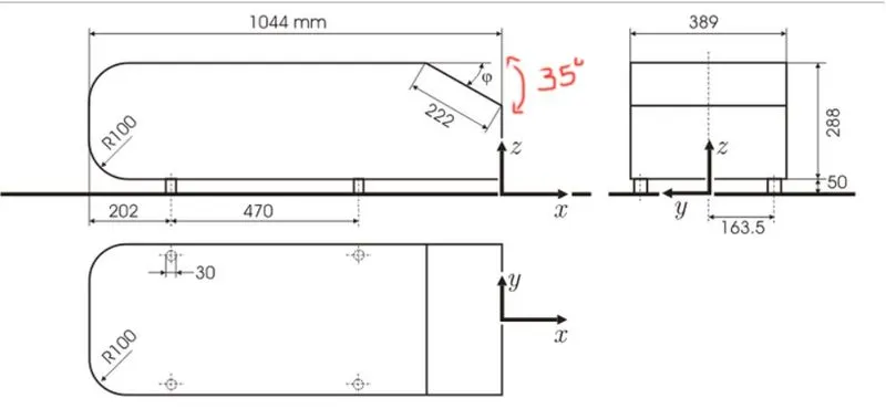
The simple geometrical shape of the ahmed body, has a length of 1.044 metrs, height of 0.288 meters, width 0.389 meters. It has a 0.5 meters cylindrical legs attached to it. The slant angle for this project is 35 degrees.
Drag and lift:
Aerodynamic drag quantifies the sleekness of the vehicle configuration. The coefficient of drag or simply drag coefficient is defined as the ratio of the drag force and the 0.5 times the product of density, square of the velocity and the frontal area exposed to the flow.
`C_d=D/(0.5*rho*U^2*A)`
`D` is the drag force;
`rho`is the density of fluid
`U`is the velocity of the car
`A`is the exposed frontal area.
The good aspect of the formula is that the coefficient donot change much with the speed, but repersents how smoothly the vehicle slices through the oncoming stream/.
The power `P` to overcome the aerodynamic drag is simply drag times the velocity.
`P=D*U`
So, less the drag, less is the power required or power consumption, more is the fuel efficiency.
The coefficient of lift or the lift coefficient is the number to model all the complex dependencies of shape , inclination, and some flow conditions.
`C_l=L/(A*0.5*U^2*rho`
here,`C_l`is the coefficient of lift.
geometry and wind tunnel :
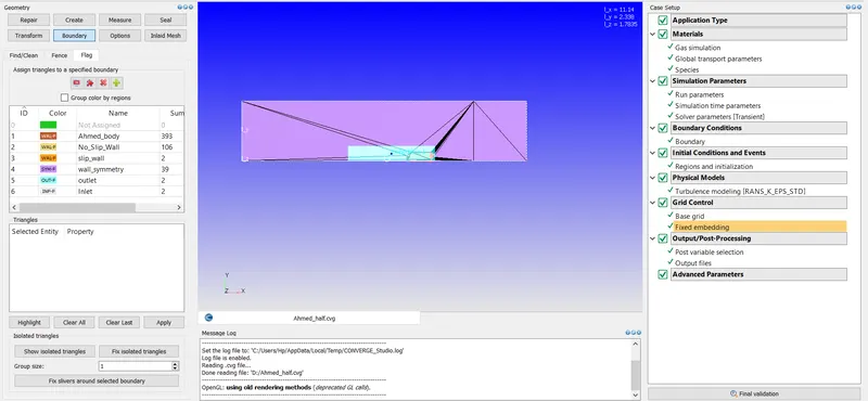
To capture the external aerodynamics, wind tunnel creation is a must. The size of the wind tunnel depends on the geometry and the inlet velocity. Generally, the length of the wind tunnel is (10 to 50) times the length of the body of the model.
For this project, the following methodolgy is used:
The boundary layer thickness formulation used here is:
`delta``delta=0.382*x/(Re_x^1.5)`
here, `delta,Re_x,x`is the boundary layer thickness, local reynolds number , and the distance where the flow is developed fully.
Local reynolds number is given by, `Re_x``Re_x=(rho*U*x)/(mu)`
In this project, the boundary layer thickness is given as , 30 mm, and the inlet velocity is 40m/s.
The frontal distance is calculated as: `1+1.6636+0.4` There is a slip region of one meter .
The lemgth of the wind tunnel is calculated as :
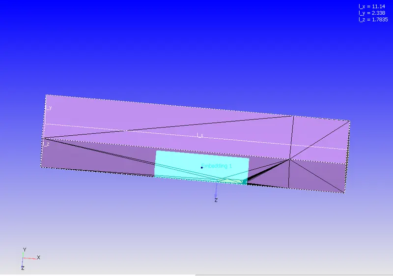
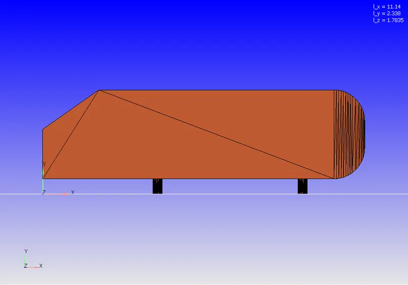
`3.06+1.044+(7*1.044)`=`11.412 m`
Case set up:
- Application type:
This is atime based simulation. This donot include any ic engine parts.
- Materials:
Under the materials tab, there are three options:
The preferred mixture selected is air. reaction mechanism is turned off and the species is turned on.
1) Gas simulation:
Equation of state = Redwich_Kwong
Critical Temperature : 133K
Critical Pressure = 377000 Pa
2) Global transport parameter:
Turbulent Prandtl number: 0.9
Turbulent scmidt number : 0.78
3)Species:
The species selected are O2 and N2.
- Simulation parameters:
1) Run parameters:
solver type is transient. Full hydrodynamic and a compressible flow simulation is carried out.
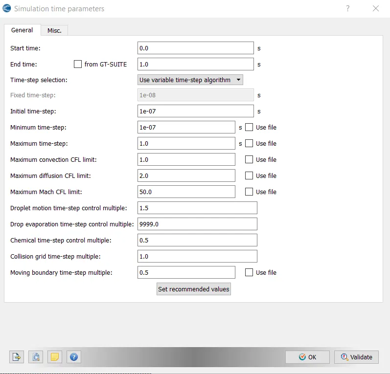
2) simulation time parameters:
Since this is a transient simulation, the end time and the start time is only in seconds.
Start time is given as 0 seconds and the end time is given as 1 seconds. The flow time is calculated as follows,
`flow time =(L)/(U)`
Calculatiing this, the value came as 2.5 seconds. Since there is computational constraint, the end time is taken as 1 seconds.
Initial time step and the final time step is 1e-07 . The maximum time step is 1 seconds.
The maximum convection CFL limit is 1 and the maximum diffusion CFL limit is 2.
3) Solver parameter:
The Navier stokes solver scheme selected is PISO
density based solver is used.
- Boundary conditions:
The boundaries created in this project are:
1) Ahmed body
2)No slip walls
3)slip walls
4) Outlet
5)inlet
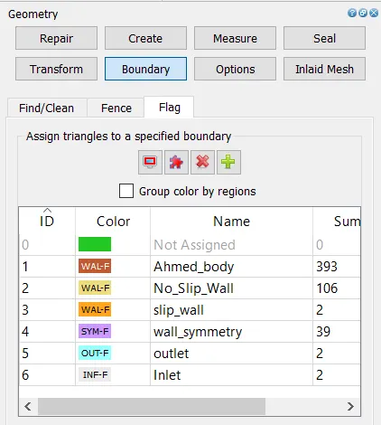
1) Ahmed body:
Boundary type : Wall
Velocity boundary conditions:
Wall motion type : stationary
Surface movement : Fixed
Temperature boundary condition: Zero normal gradient (NE)
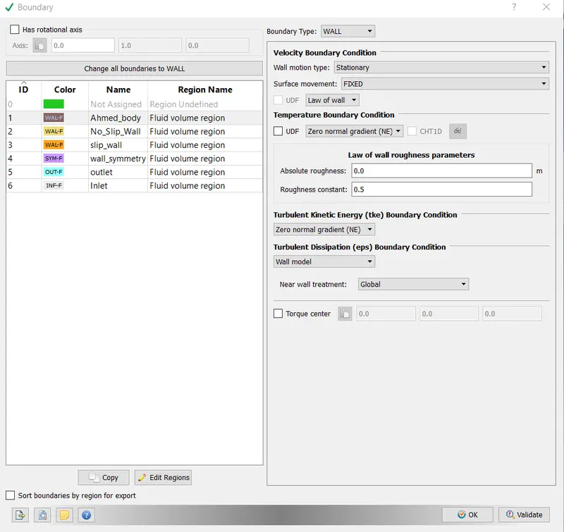
2) No slip walls:
Boundary type : Wall
Surface movement : fixed and the surface type is no slip
The temperature boubdary condition is provided asbZero normal gradient (Neuman boundary condition)
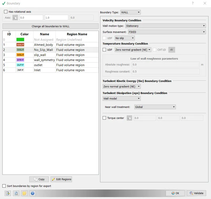
3) Slip wall:
Boundary type : Wall
Surface movement : fixed and the surface type is slip.
The temperature boundary condiotion is Zero normal gradient (Neuman)
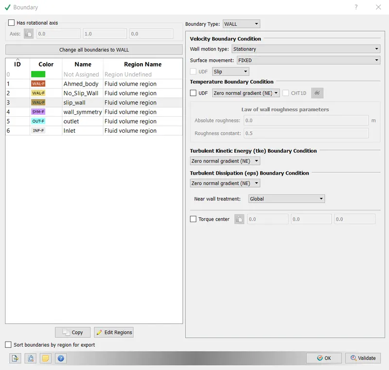
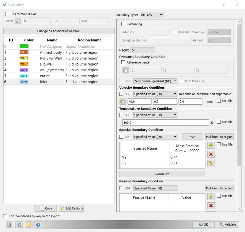
4) Inlet:
Boundary type : Inflow
Pressure boundary condition: Zero normal gradient.
Velocity boundary condition: Specified value(DI)
the inlet velocity is assigned as -40m/s
The temperature boundary condition is Specified value(DI) and is assigned as 300K
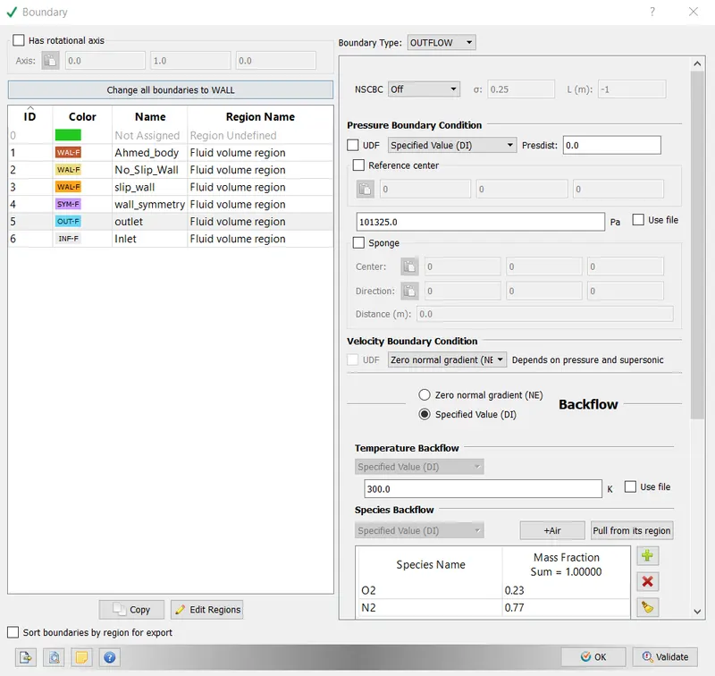
5) Outlet:
Boundary type : Outflow
Pressure boundary condition: Specified value(DI)
It is assignmed as 101325 Pa
The velocity boundary condition is Zero normal gradient (NE)
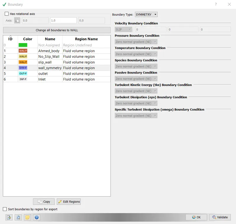
6) Symmetry walls:
Symmetry boundary condition prevails
- Regions and initializations:
A fluid volume region is created with temperature as 300 k, pressure as 101325 Pa, and the inlet velocity as 40 m/s. All the boundary flags are assigned to this region.
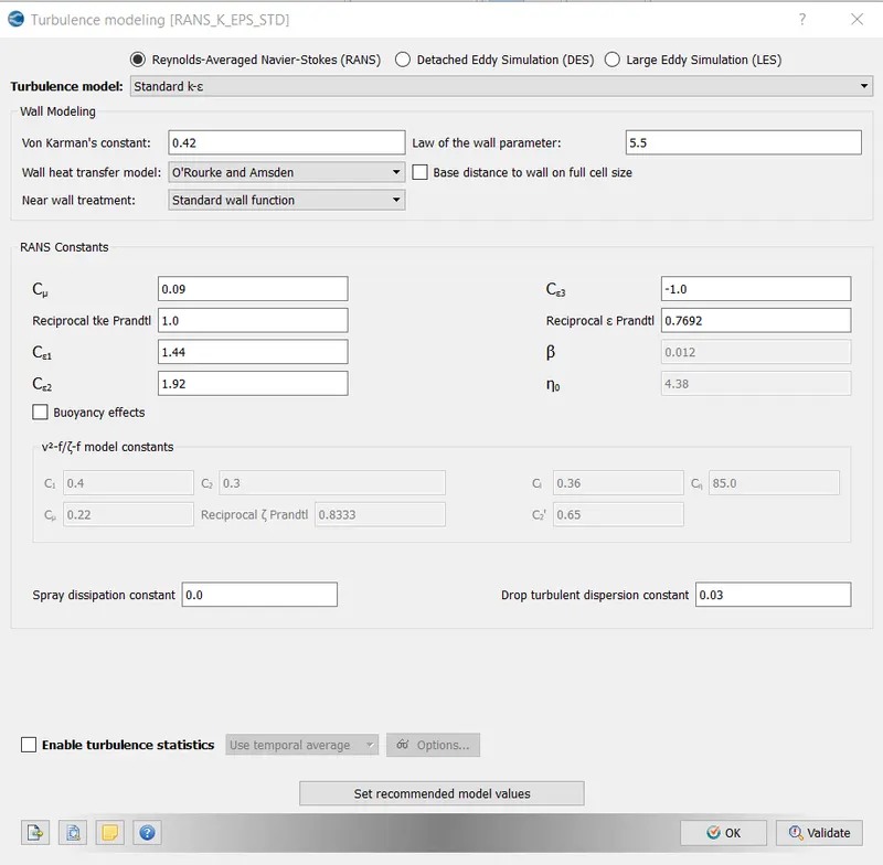
- Physical models:
Under the physical models tab, the turbulence modelling is done only.
Turbulence model:
- Grid control:
Two types of grid control is monitored, Base grid and fixed embedding to refine the mesh in the regions of interst.
Base grid:
From the y+ values the base grid can be calculated. In this case the base grid size selected is 0.1 meters in all the three co ordinates.
Fixed embedding:
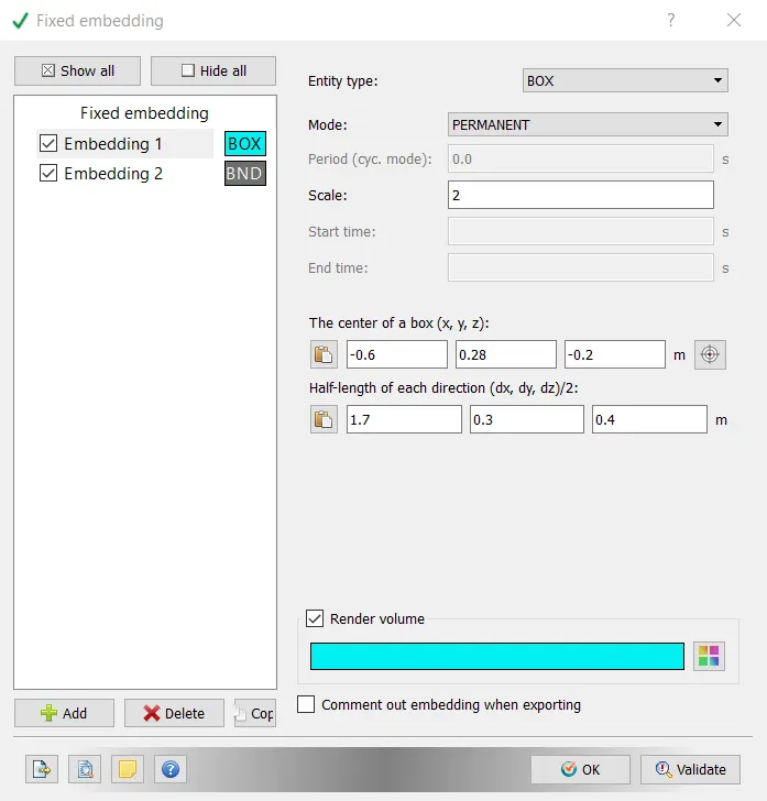
1) embedding 1:
Entity type : box.
mode : permanent
scale : 2
2) Embedding 2:
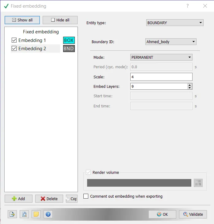
This embedding is provided to the Ahmed body. Entioty type is boundary. Mode : permanent. The total nu,ber of embedded layes is 9 and the scale is 4.
- Post processing and output files:
Since the external aerodynamics profiles are to be seen, the wall boundary is checked. Y+ value is also to be monitored.
To run the simulation:
mpiexec.exe -n 4 converge.exe restricted this command is used . The 4 attributes to the number of processors .
Results:
- Line plots:
1) The cell count:
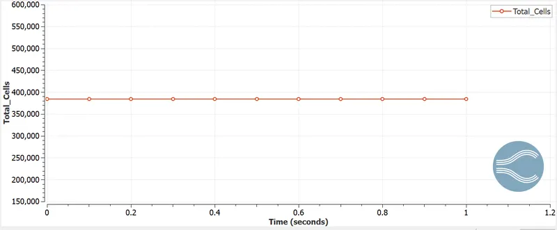
The cell count is 384000.
2) drag force:
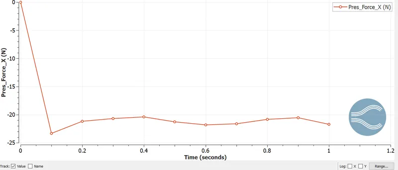
The drag force plot can be obtained from the boundary1.output files. The drag force obtained is 21.7179 N . The orientation is that the inlet is to the negative of a axis.
3) Lift force:
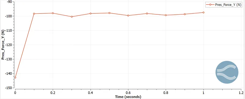
The lift force obtained is 104 N.
To obtain the contours of velocity and pressure, Paraview software is used
- Mesh generation:
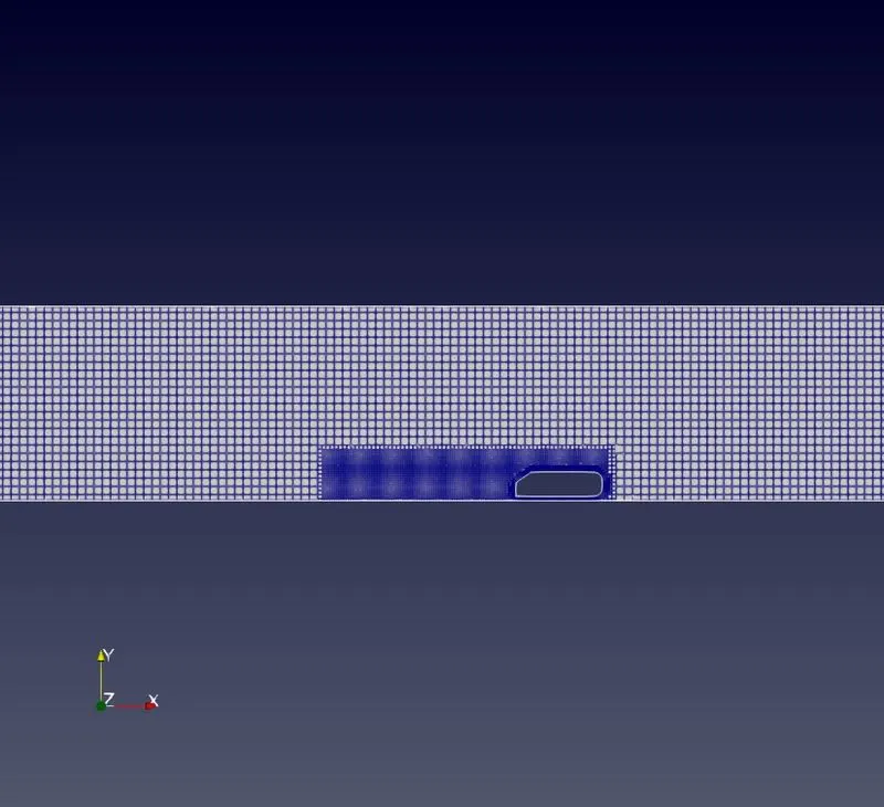
From the 3D geometry obtained, A slice is cut with direction as normals along the Z axis. This cut plane is created to visualize the contours properly.
- Velocity contours:
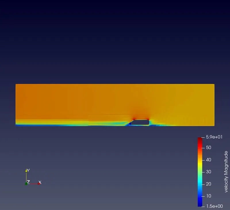
The velocity contours on the Ahmed body, is as follows. Using the multi block inspector tab, all other componemts of the 3D geometry is omitted keeping only the half ahmed body.
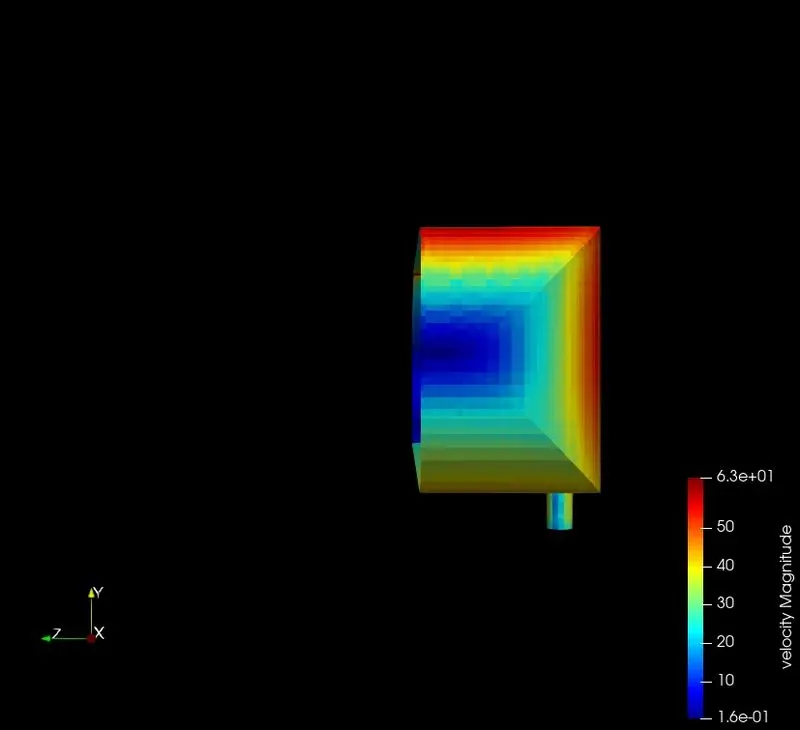
The velocity distribution on the full wind tunnel is visulazed as follws:
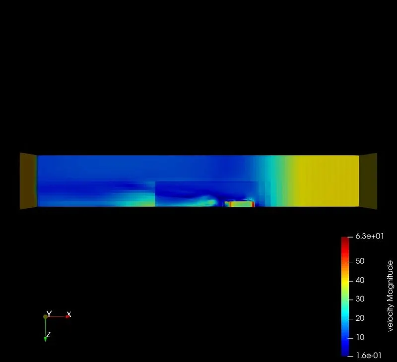
- Velocity vectors:
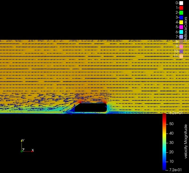
By using the glyph options, vectors along the velocity can be visualized. The region of circulation and the flow separation can be visualized.
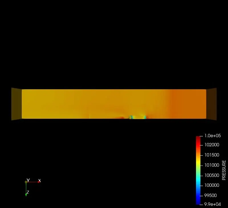
- Pressure contours:
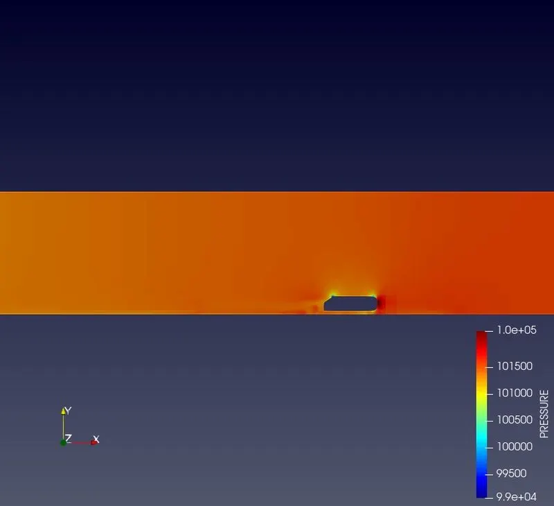
Pressure distribution on the ahmed body:
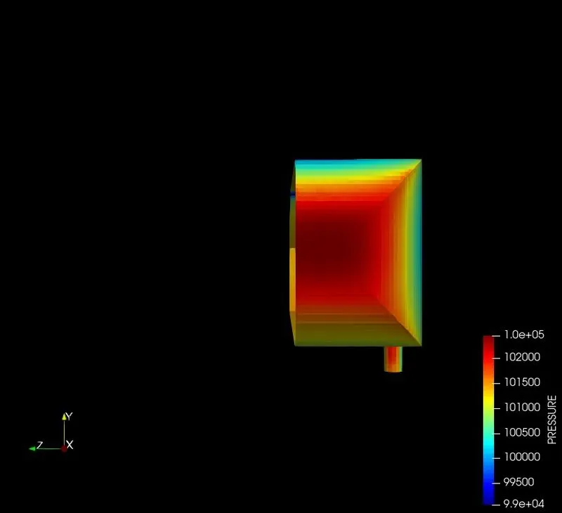
On the complete wind tunnel:
The animation of velocity contour is :
- Projected area in paraview:
Steps:
1) Allign the geometry in proper view, along the incoming flow.
2) Select the 'select cells upon' selection, draw a box on the desired face.
3) Next we need to extract the selection. Use extract selection. The projected area is reduced by this.
4) We need to do another transformation, to transform it into a 2D projection. using, filters, search the transformation tool, click apply. After this a box is created around the previously created transformation. The scaling factor may be changed manually.
5) To get the specific value, use the tool 'integrate variable' the propjected area is obtained.
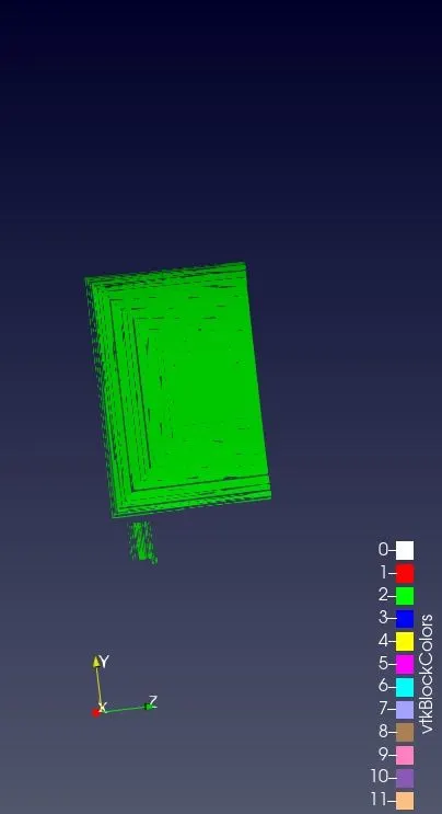 This is the projected area.
The projected area obtained is , or the frontal area obtained is 0.0495 m^2.
The cofficient of drag and coefficient of lift can be calculated using the this value of the projected frontal area.
`rho` of air at 300K is 1.225 kg/m^3
`C_d=(D)/(0.5*rho*V^2*A`
From this putting the above values, the coefficient pf drag obtained is 0.41.
C_l= -0.78
- Average y+plus value:
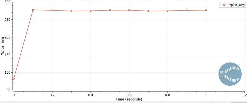
The y+ value should be between the range of 30 and 300. In this case it is 270 .
y+ :
The wall functions rely on the universal law of wall which basically states that the velocity distribution very near to a wall is similar for almost all turbulent flows. One of the most prominent parameters when judging the applicability of wall functions is the so-called dimensionless wall distance y+.
`y+=y*u_tau/(nu)`
`u_tau`is the frictional velocity,`y`is the average distance from the wall, `nu`is the frictional velocity.
Conclusions:
- Examining the velocity profile it is seen that there is a region where there is circulation and the region is called wake region. This region causes drag.
- The negative lift force says that it is down force. This attributes to the fact the model stays at the ground.
- The shape of the body or the passenger vehicle may be optimized to reduce the lift force .
- To get more better results, finer grid may be created that may require more computational resources.