Simulation of flow around an Ahmed Body
AIM:
The aim of this project is to model an Ahmed body and simulate the flow over it in converge.
OBJECTIVES OF THE PROJECT:
- Create the CAD model using any CAD package.
- Setup a Coarse CFD simulation.
- Setup the virtual wind tunnel.
- Apply the right boundary conditions and solver settings.
- Generate an animation of the velocity distribution on a cutplane which cut the Ahmed body model into two symmetric pieces.
- You need to show an animation of the pressure distribution on a cutplane which cut the Ahmed body model into two symmetric pieces.
- Post-process the coarse mesh results and extract the x component of velocity along a line.
- Calculate the steady-state drag force value.
- Calculate the drag co-efficient using paraview.
THEORY
What is an Ahmed body?
The Ahmed body is a geometric shape first proposed by S. R. Ahmed and Ramm in 1984. The shape provides a model to study geometric effects on the wakes of ground vehicles (like cars). It is used to validate the CFD solvers. The results of airflow over this body were captured using the wind tunnel experiments and the CFD solver results are compared with these experimental results to find out the accuracy of the solver.
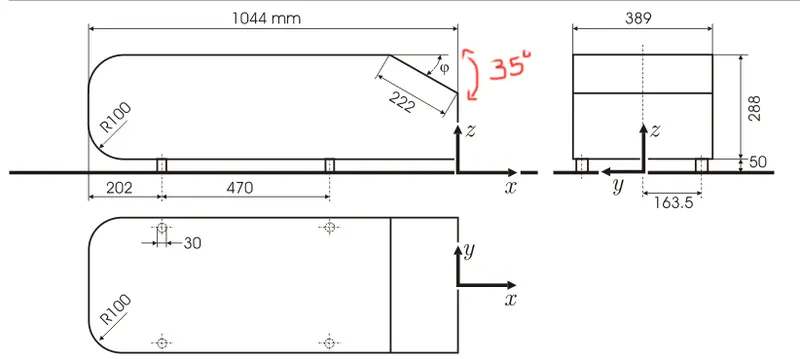
The geometrical details of the Ahmed body are in this figure.
PROCEDURE:
Generating the CAD model
Generating the CAD model can be done in any CAD package. I used FreeCAD to generate the STL file. First extruded the box with 1044 and 389 mm over a length of 288 mm. Then added the 4 cylinders, 30 mm dia and added the fillets using the arc commands and the final part is as shown.
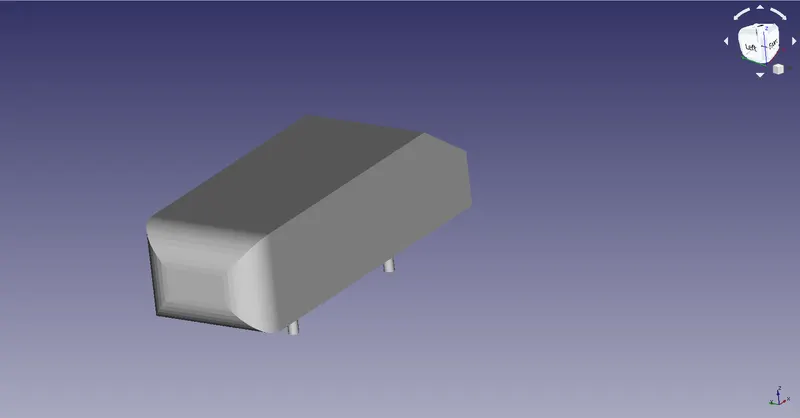
While generating the model, I ensured that all dimensions are arrested and accurate. We can then export this in the form of an STL file which is then fed to Converge Studio.
We import the STL file into converge.
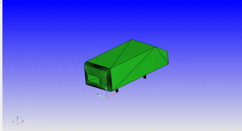
Once the geometry appears, we need to check the geometry units. We can do this by going to the Left-side geometry panel > Options > check the boundary box.
Converge uses an MKS system, while the geometry would have been created in MMGS, so we need to transform the body to a smaller scale to get meaningful results.
If the boundary size is in the range of 100meters we can scale it by geometry panel > Transform > Scale > give a scaling factor of 0.001. And the geometry will come to a range of 0.1 m.
Note that for the experiment the origin was at the centre of the bottom-most edge on the back of the Ahmed body (see the above picture for reference).
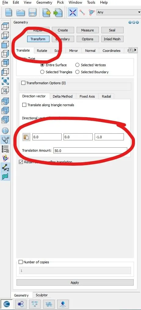
For our convenience, we translate the Ahmed body such that the origin is exactly as shown in the above image. We can do this by using the translate tool in the transform tab.
To observe the flow over an Ahmed body we create a virtual wind tunnel.
We do this by creating another geometry on this.
But before we create the wind tunnel, we need to know the dimensions of the wind tunnel.
We know that the ground has a slip region. We can assume it as 1m
Also, we know that the flow must have a boundary layer thickness of 30mm at 400mm before the Ahmed body.
For the boundary layer to develop a thickness over a flat plate we have the formula
`delta = {0.382x}/{Re_x^{1/5}}`
The Reynolds number for a characteristic length is given by `Re_x = frac{rho*V*x}{mu}`
we know that delta is 0.03 m therefore from the above two equations
`0.03 = frac{0.382x}{{frac{rho*V*x}{mu}}^{1/5}}`
The Ahmed body experiment was conducted at an air velocity of 40m/s
Plugging in the known values such as the air density and dynamic viscosity and performing the mathematical operations
we get `x = {frac{40}{(1.273)^5*1.562}}^{1/4}`
Upon solving it `x = 1.6636 m`
So the frontal distance should be `1.0+1.6636+0.4 = 3.0636`
The distance after the Ahmed body should be 5 - 10 times the characteristic length but 10 times the characteristic length requires more computational time and power hence we reduce it to 6 times to accurately capture the wake produced.
Now the total length in the x-direction would be 3.0636 + 1.044+ 6*1.044 = 10.37(approx) we round it off to 10 m
In the z-direction, the total length should be at least 5 times but due to computational restraint we reduce it to 2 m
we keep the same length for y as well, Y direction length is 2 m
To create the wind tunnel, we create a box using the create option and input the dimensions as 10 for x and 2 for y and 2 for z and for the Ahmed body to be on the floor of the wind tunnel the centre of the wind tunnel must be calculated based on wind tunnel conditions and frontal distance.
Once the wind tunnel is created we delete the bottom face and create two vertices such that those two vertices are 1m distance from the inlet face. We then patch the bottom of Ahmed body with these two vertices using the ordered vertex list option in the patch tool in the repair tab and create a new bottom face. This would look something like this
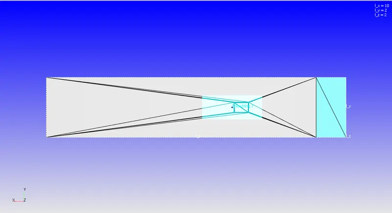
Note that the side faces also should be reconstructed else this would result in an intersection error. Once the patching is done we check the normal direction. The normals should be pointing towards the fluid domain, If the normals are pointing the opposite they can be corrected using the normal option in the transform tab.
Once the Diagnosis is all green we can proceed to flag the boundaries. The boundaries need to be flagged as shown.
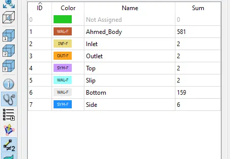
- Now left-click on a boundary name and select the triangles on the geometry to assign those triangles to the boundary. Repeat this process for both the boundaries created.
- We can make sure that all the boundaries are assigned by checking the Not Assigned (Boundary ID 0), If the triangles in this boundary are none then all the triangles are assigned to the created boundaries.
We move on to setting up the case
The type of simulation is time-based and with the default gas simulation constants and global transport parameters, we input the species as N2 and O2.
Here we set up a transient case. The steady-state solver is not suitable for this kind of simulations
In the miscellaneous tab uncheck the use shared memory option and uncheck the solve for species option and click on ok.
In the Simulation time parameters enter the following value
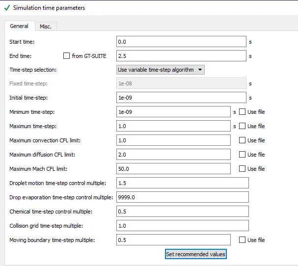
The Time required is calculated using the flow-through time. Since the length the air would travel is 10m and the velocity is 40m/s it would require 0.25s for the air to pass through the WindTunnel. But we take ten times this flow and we end up with 2.5s
In the solver parameters section select the Density-based option. Upon selecting this all the parameters in the solver parameters section will be selected automatically
Now before we go into the boundaries option click on regions and initialisation. Click on add new region. Right-click on region 0 and rename it to high pressure. On the left side near the species click on + and add air and select the temperature as 300k and pressure as 101325pa and velocity to 40m/s.
Now we apply the boundary conditions as follows
All the regions will be set to region 0. And the type of boundaries is as follows.
| Ahmed Body | Wall - Law of the wall |
| Inlet | Inflow, velocity-Dirichlet, Pressure -Neuman |
| Outlet | Outflow, Velocity-Zero normal gradient, pressure-Specified value-101325 |
| Top | Symmetry |
| Slip region | Wall - Slip |
| Bottom | Wall - Law of the wall |
| Side | Symmetry |
We could've gone for No slip in the bottom face but for no-slip, the bottom layer of cells will be treated as a viscous sublayer. For a viscous sublayer, a very small grid size is important. Since we can't afford a smaller grid size we use the Law of the wall BC. This uses logarithmic interpolation to solve the Bottom face.
And make sure the inlet boundary velocity is a specified value of 40 m/s.
In the physical models > Turbulence modelling select the RANS option and select Komega SST and press ok.
In the Grid Control,> select Fixed embedding and press ok
In the Base Grid,> set the x, y, z sizes to 0.06 m and click ok.
In the fixed embedding add two embedding as shown
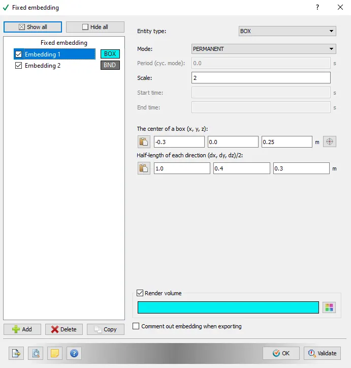
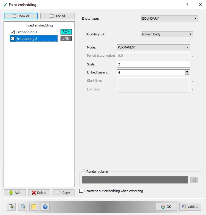
If we don't add the fixed embedding to the boundary it will result in Converge stopping after writing the first post output file.
We then select the output file settings. The Output files settings are as follows
The wall output is set to BOUNDARIES ONLY.
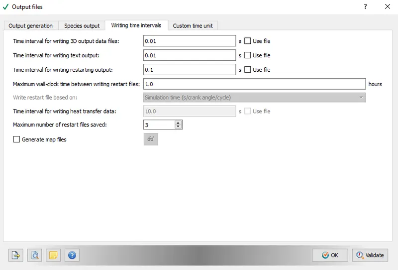
Once all the setup is done we do the final validation. Once every tab is green we export the files using the export input files option.
We then run the simulation using the CYGWIN terminal. In the terminal, we navigate to the folder that contains the input files enter the following command.
"mpiexec.exe -n 4 converge.exe restricted </dev/null> logfile.txt &"
- mpiexec.exe is the message passing interface executive file.
- -n 6 represents the number of cores to be used for running the simulation.
- converge.exe is the converge file that runs the simulation.
- restricted limits the total number of cells to 5,00,000
- </dev/null> logfile.txt is to create a log file that can be used to track the simulation.
- & To keep the Cygwin terminal active for other commands
"tail -f logfile.txt"
This command tracks the log file and displays the content of the log file in the terminal.
The simulation might take several hours based on parameters like Hardware, grid size, time for which the simulation needs to be run. Once the calculations are finished exit the Cygwin terminal.
POST PROCESSING:
In the input file directory, a new folder will be created with the name "output". The post output files are stored here. We navigate to the post-processing module in Converge Studio and select this output and convert them into "Paraview-inline binary format" or "Ensight" format.
Once this is done we open the results in paraview. We reduce the opacity of the side walls to see Ahmed body inside the wind tunnel.
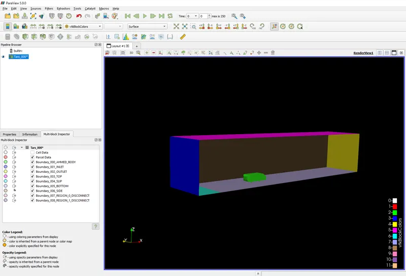
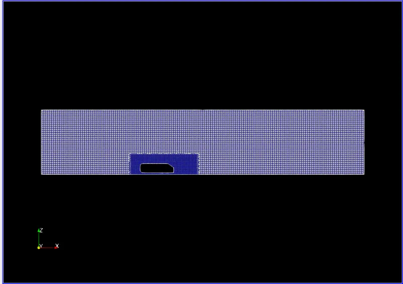
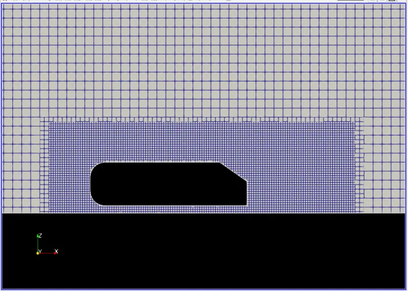
We can see that each boundary has been assigned with different colours. We then take a slice of this with Y-axis as the normal. This would cut the Ahmed body in symmetric and we can observe the mesh using the surface-with-edges option.
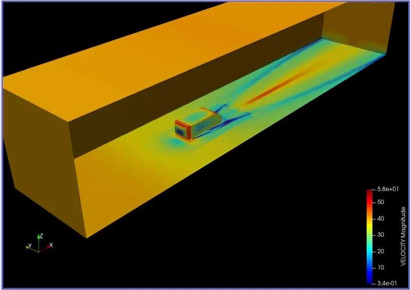
Instead of solid colour, we can set it to velocity and pressure to see contours like these
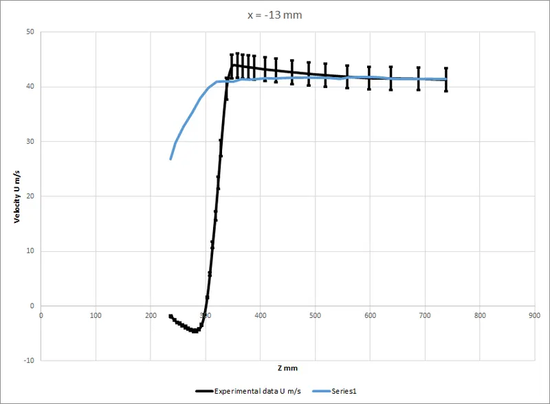
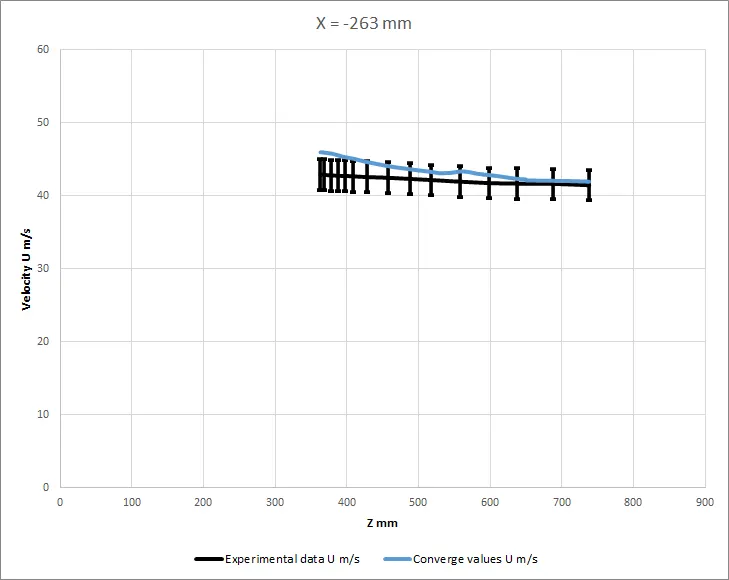
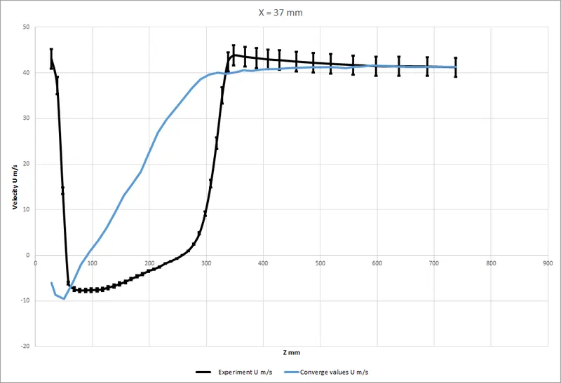
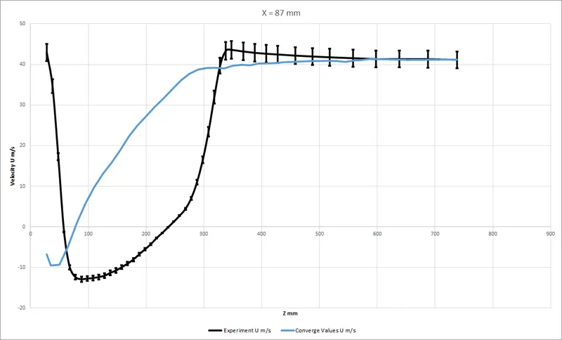
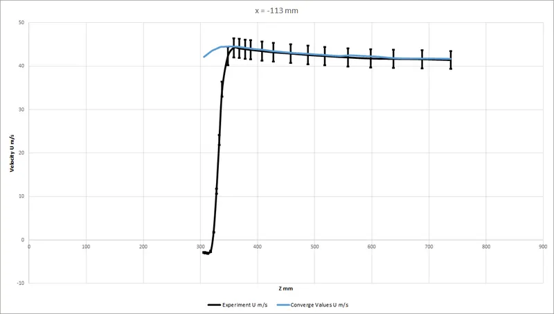
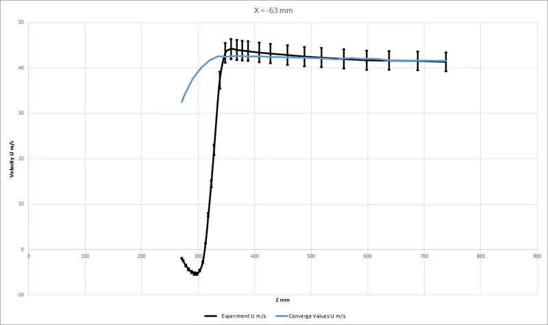
We have some experimental data from "S. Becker, H. Lienhart, C. Stoots, ERCOFTAC workshop 9.4(2000): LDA-Measurement". They collected the velocity along x-direction at different locations along the X and Z axes using probes And plotted some graphs with that data. This data can be found here. We are going to do the same in a virtual system.
Using the plot over line option in paraview we can extract the velocity in the X direction at different locations along the X and Z axes. The plot over line command plots the Z location Vs velocity along X for different X locations. We use the export scene option to export this plot data into an excel sheet.
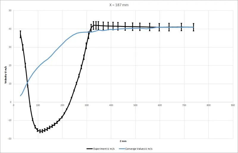
We take both the experimental data and the simulated data and plot them in a single graph we get the following graphs for different locations.
@ x = -13 mm
@ x = -263 mm
@ x = 37 mm
@ x = 87 mm
@ x = -113 mm
@ x = -63 mm
@ x = 187 mm
@ x = 137 mm
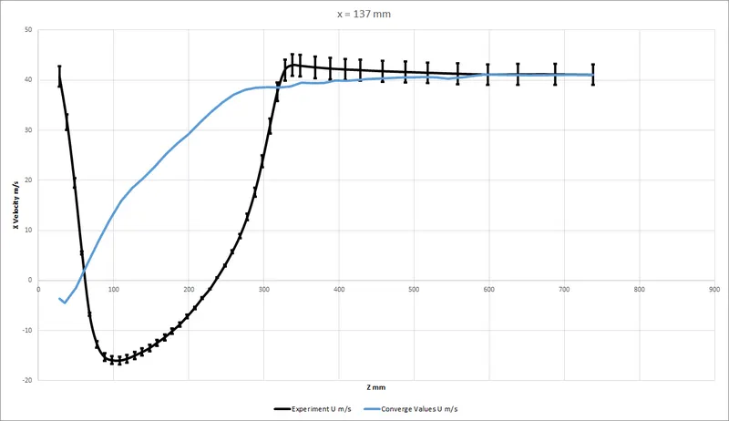
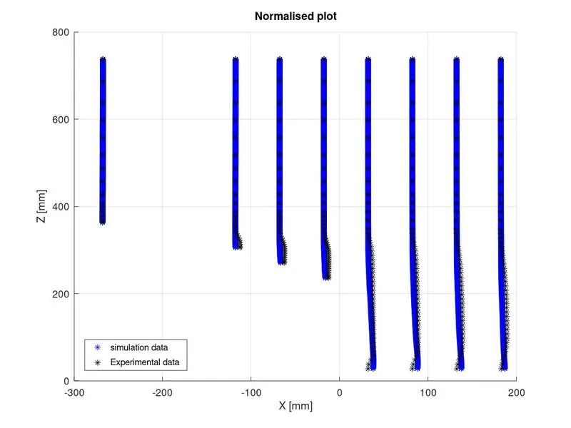
The spikes in the above graphs indicate an error percentage of 5%. The above plots are for different locations along X. We can to normalise the above data using octave and put them in a single graph it would look like this
Now that we have got all our data we calculate the lift and drag coefficients.
we know that lift force `F_l = 1/2C_l*rho*A*V^2`
Where `C_l`is the Lift coefficient and A is the wing Area in terms of aeronautics. This is an area upon which the lift is produced by Bernoulli's principle. This is the product of the wingspan and chord length. In our terms, it is `(1044*398) mm^2`.
Drag force `F_d = 1/2*C_d*rho*A*V^2`
Where `C_d` is the drag coefficient and A is the frontal area. This can be extracted from paraview
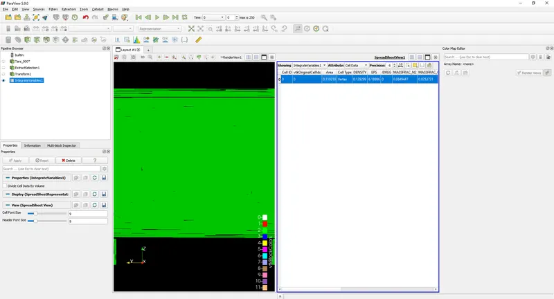
It is nothing but `(389*288)mm^2`
we need to find out the drag and lift forces. These can be extracted from Converge using the line plotting module.
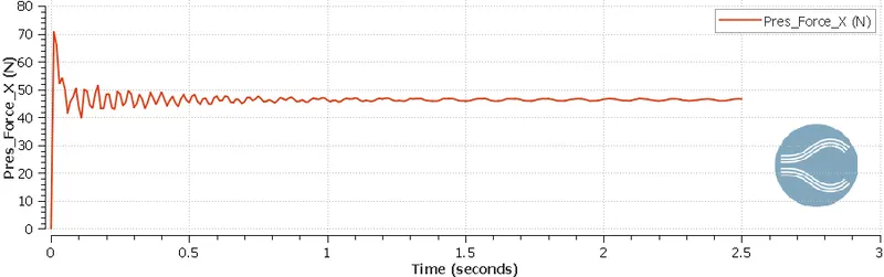
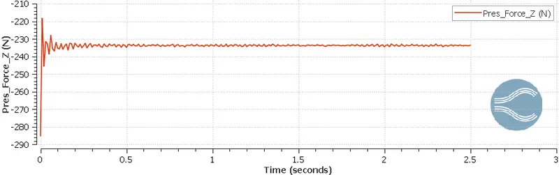
This plot data can be extracted using the preview plot data option in the converge line plotting module.
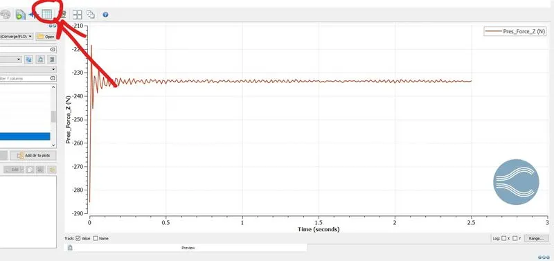
Once the drag and lift force values are extracted we can use octave to calculate the mean of these values. This will be our drag and lift forces
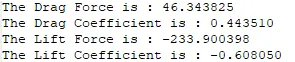
we plug in these values in the above equations to find out the drag and lift coefficients.
The results are as follows.
CONCLUSION:
- From the graphs, we can see that the probes at the negative location are matching well with the experimental data compared to the probes on the positive side.
- On the positive side, we can see that the error percentage in the graphs is greater than 5%. This is because of the grid size. We can reduce the grid size or simulate only one symmetric half with reduced grid size.
- The error on the positive side is greater because of the Drag produced on the rear side of the body. The rear side is positive from origin.
- To capture this wake region correctly a smaller grid size and greater computational power are required.
- From the Velocity contour, it is observed that after passing through the geometry there is a region where recirculation happens this region is called as wake region. Due to this low pressure, the air at the front tries to come back which increases the drag.
- The air after exiting the cylindrical pillars forms vortices. These vortices can be observed from the top view.
- It is also observed that the lift obtained is negative which means that it is downward force. This force helps racing cars to stay on the ground. But for a low-efficiency vehicle such as a truck, this force is not desirable. Hence the shape of the truck/trailer will be optimized to reduce the negative lift.
REFERENCES: