Hyper elastic Material Modeling in LS-Dyna

Objective: To calculate the Mooney Rivlin and Ogden material constants and compare them using stress-strain data from a Dogbone specimen tensile test with 100 percent strain.

Procedure:

• The stress-strain points are written in Excel and saved in .csv format to load into the LS-Dyna.

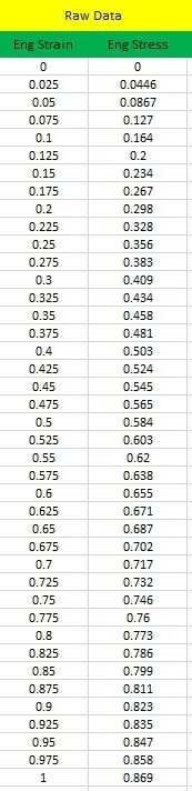
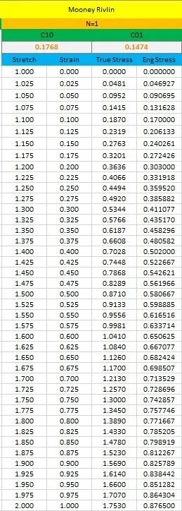
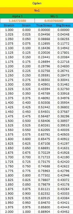
Fig 1: Provided engineering stress and strain values.

• Import the dog-bone specimen in LS-Dyna.

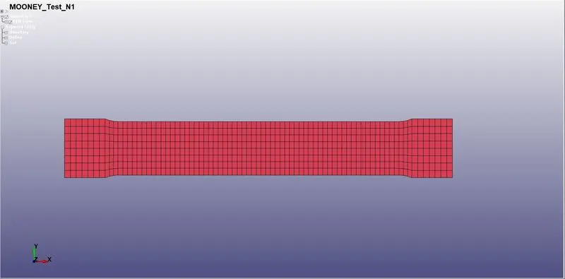
Fig 2: Specimen.

• Assign a proper part name to the auto-created part.
• Create a Shell section card with ELFORM of 2 and a thickness of 1.5mm.

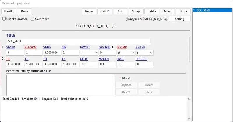
Fig 3: Section card is defined.

• Mat077_H HYPERELASTIC_RUBBER card is created with the following properties:

Density: 0.001.

Poisson's Ratio: 0.4995.

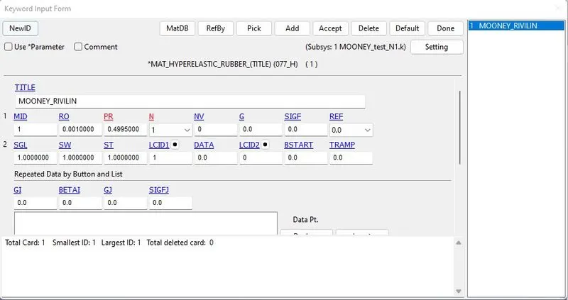
Fig 4a: Mooney Rivlin material card is defined with N=1.

FOR OGDEN MATERIAL MODEL:

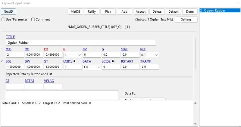
Fig 4b: Ogden material card is defined with N=1.

• Hourglass card is added to control the hourglass formation in the shell elements.

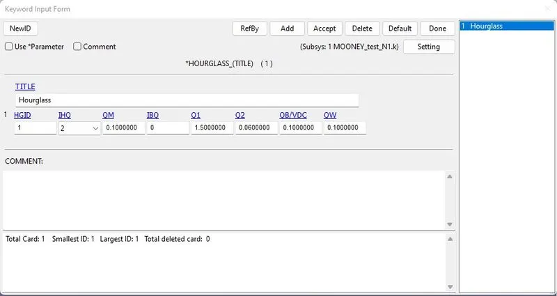
Fig 5: Hourglass card is defined with Flanagan-Belytschko viscous form.

• Section, material and hourglass is assigned to the specimen part created earlier.

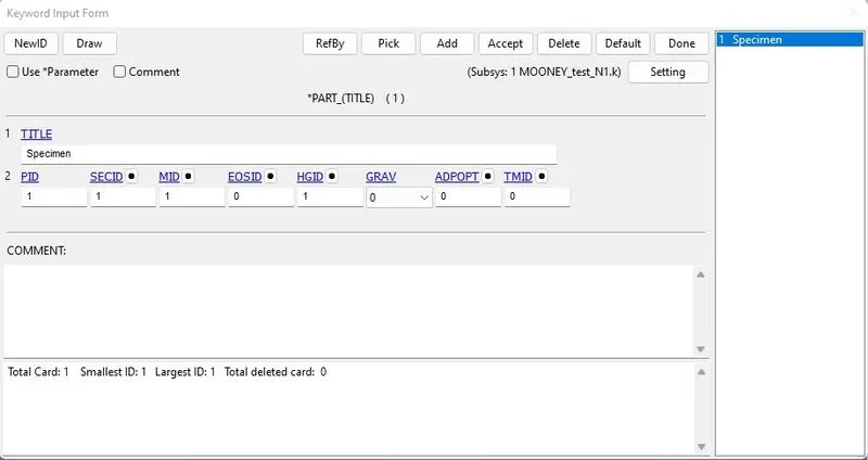
Fig 6: Material, section and hourglass is assigned to the part.

• To emulate the tensile test in LS-Dyna, appropriate boundary conditions must be provided.
• The left end edge nodes of the dogbone specimen is constraint in x-translational direction.

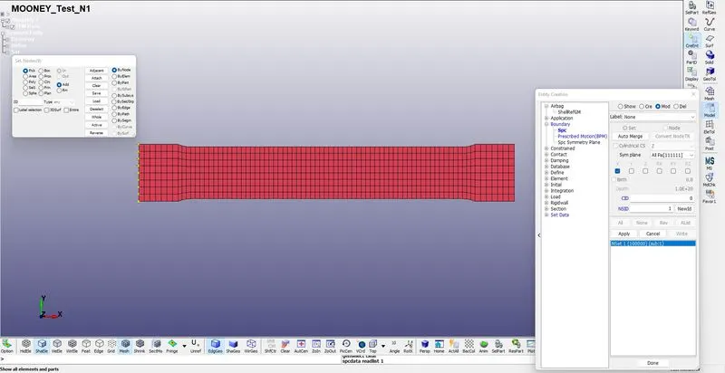
Fig 7: The left end nodes are constraint in x direction.

• Mid-nodes of both the ends are constraint in y direction.

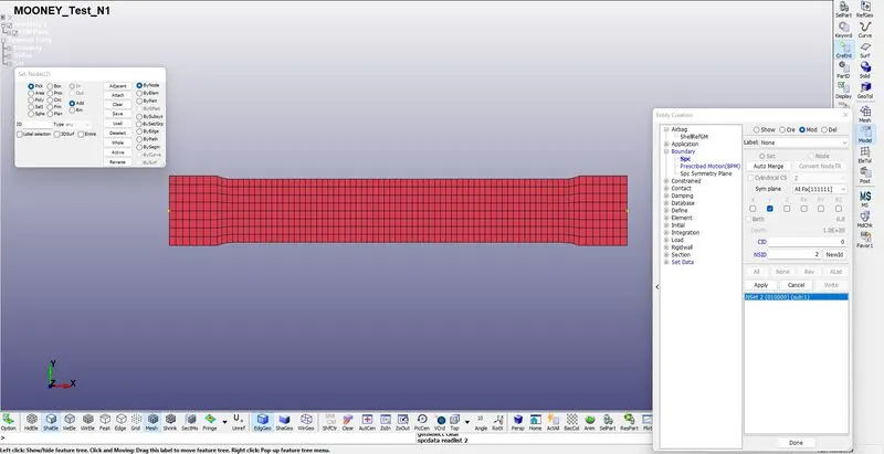
Fig 8: Mid-nodes are contraint.

• The right end nodes are selected and created a new Node_set to which displacement boundary condition is applied.

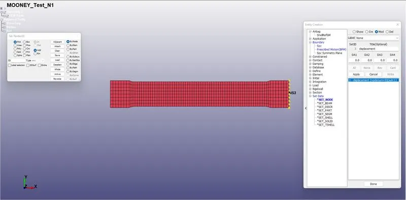
Fig 9: Node set is created to assign displacement boundary condition.

• PRESCRIBED_MOTION_SET boundary condition is added with DOF 1 and VAD 2.

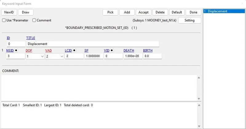
Fig 10: PRESCRIBED_MOTION_SET card is defined.

• The stress-strain points which were saved earlier are loaded into the curve card.

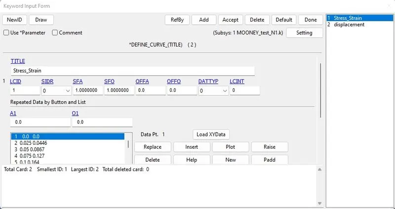
Fig 11: The curve points are loaded into the curve card.

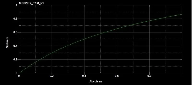
Fig 12: Stress-strain curve.

• Displacement curve is also defined.

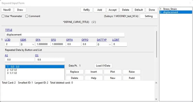
Fig 13: Displacement is defined.

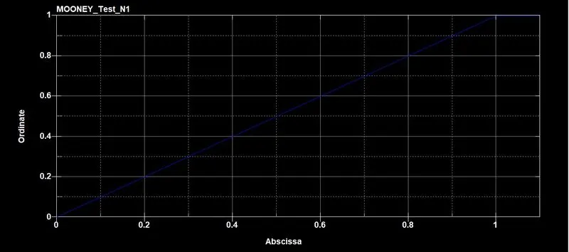
Fig 14: Displacement curve.

• To solve this particular simulation implicit solver is chosen. To define the implicit solver, specific implicit keywords must be included.
• IMPLICIT_AUTO, IMPLICIT_GENERAL, IMPLICIT_SOLUTION, and IMPLICIT_SOLVER keywords must be added from the control deck.

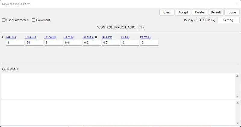
Fig 15: Implicit_auto card is defined.

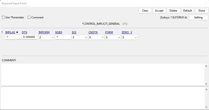
Fig 16: Implicit_general card is defined.

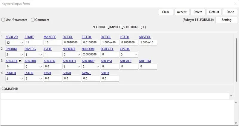
Fig 17: Implicit_solution card is defined.

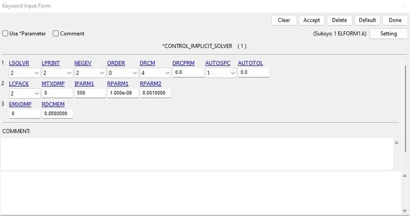
Fig 18: Implicit_solver card is defined.

• The ASCII_option keyword from the DATABASE deck is used for the output requests, and the GLSTAT option is checked.

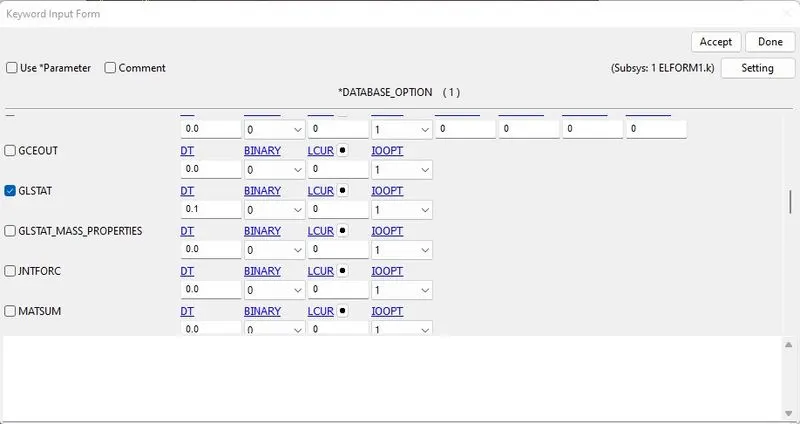
Fig 19: Output requests are defined.

• The BINARY_D3PLOT keyword from the DATABASE deck is used for the plots, and a DT of 0.1 is entered.

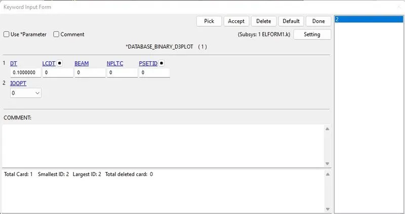
Fig 20: Plots at time intervals are defined.

• Finally, the TERMINATION keyword from the CONTROL deck is used to define the end time of the simulation.

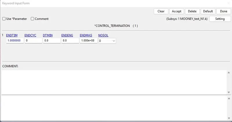
Fig 21: End time for the simulation is defined.

• With all these keywords included, the deck is fully defined and is now ready to solve.

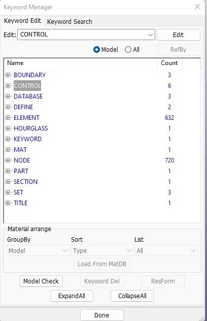
Fig 22: Fully defined deck.

• Open the Start LS-Dyna analysis, browse the keyword file, and hit run to run this keyword file.

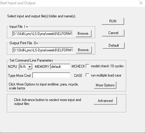
Fig 23: LS-Dyna analysis browser.

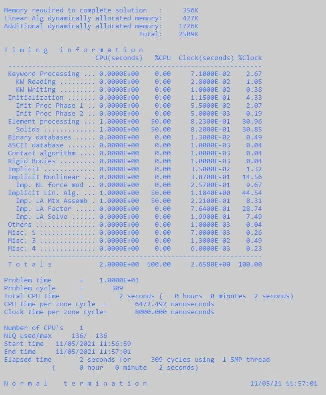
Fig 24: Successful completion of solving.

Results:

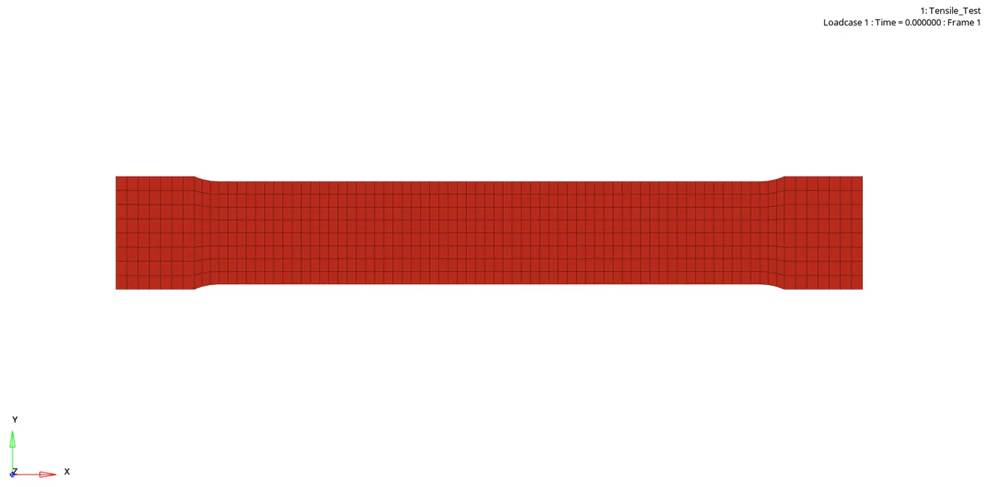
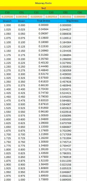
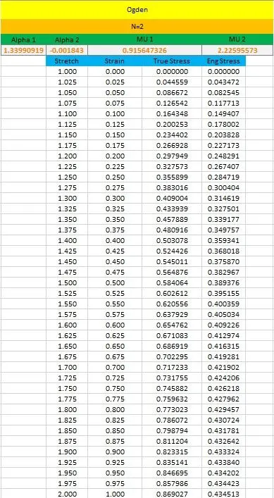
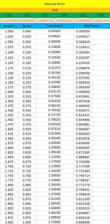
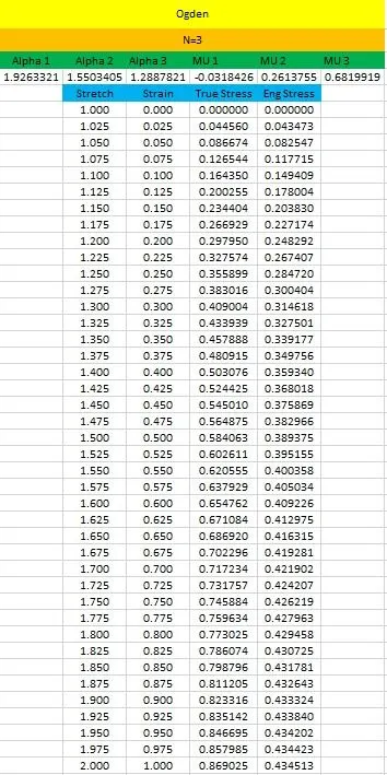
• In MAT_077 card and MAT_077_O material cards, we have to simulate with varying N1, N2, and N3 number constant to solve and extract the true stress and true strain.

CASE 1: N=1

CASE 2: N=2

CASE 3: N=3

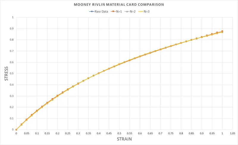
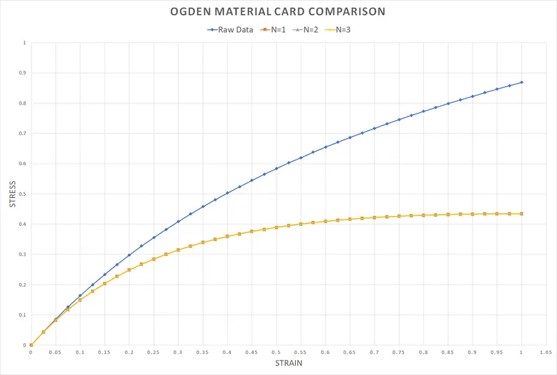
Conclusion: Calculated the Mooney Rivlin and Ogden material constants and compared both using stress-strain data from a Dogbone specimen tensile test