Week - 10 Hyperelastic Material Models

AIM: To determine the Mooney Rivlin and Ogden material constants and compare using stress-strain data with 100% strain.

Modelling Procedure:

Units: g-mm-ms-N-MPa

1. Introduction

When a material is subjected to external deformation, we know that its constitutive relationship describes its behaviour. Various constitutive relations can be used to represent various material behaviours. Hyperelastic materials, unlike any other material, are path independent, the stress update is not computed sequentially. St. Venant–Kirchhoff material, for example, provides a linear connection between stress and strain that is a straightforward extension of the one employed for linear elastic materials. Unfortunately, because most materials have a nonlinear relationship for large deformation, this model only produces useful findings when the strains are minimal.

2.  Unit Conversion:

Since for the simulation 'g-mm-ms-N-MPa' was followed, it was essential to maintain dimensional homogeneity. Thus, the stress was represented in terms of 'MPa' and the density was represented in terms of `(g)/(mm^3)`.

.  Stress vs Strain Curve for Material Model:

Usually, the True stress vs True strain curve defines the material behaviour but experimentally, engineering stress vs engineering strain curve is obtained. Following relations can be utilised to convert the curve from engineering stress-strain to true stress-strain value. 

True Strain = ln(1+Engineering Strain)

True Stress = (Engineering Stress)* exp(True Strain) 

But to define the material properties in MAT 24 material model, the stress-strain curve needs to be defined in terms of Effective Stress vs Effective Plastic Strain. So,

Effective Plastic Strain = (Total true strain) - (True stress/E)

4.  Numerical Modelling Methodology:

4.1 Material Model (MAT 77)

The given dogbone specimen was imported and the material properties were defined as follows:

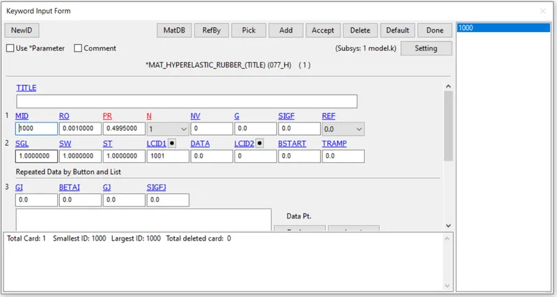
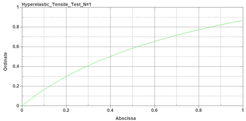
4.2 Material Properties: the material properties were defined using the experimental stress-strain graph using the Define_curve option.

  

Density: 0.001 `(g)/(mm^3`

Poisson's Ration: 0.491

4.3 Element Formulation

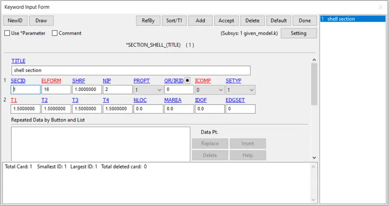
Fig: Element Formulation adopted for the simulation

4.4 Boundary Conditions

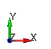
Fig: All the DOF was constrained except in Y-axis to facilitate the contraction of the material on application of tensile load. 

Fig: A node-set was created to define the displacement motion to the model from another end.  

Fig: Two central nodes along the s[ecimen were constrained in the Y-axis as it is known that there will be neither contraction nor expansion along the neutral axis of the specimen.   

4.5 Control Conditions:

Implicit_Auto card - was included to automatically adjust the time step during the simulation. 

Implicit_General - was defined to specify that the simulation is needed to be carried out using Implicit Formulation. 

Implicit_Solution - the card was invoked to specify that a non-linear solution is expected as the simulation included plasticity and failure on the application of load. 

Control_Energy  - this card was included and HGEN was set to '2' so that Hourglass energy is calculated and included in the solution. 

  

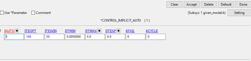
Fig: Control_Implicit_Auto Card

 

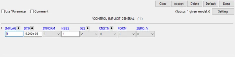
Fig: Control_Implicit_General Card

 

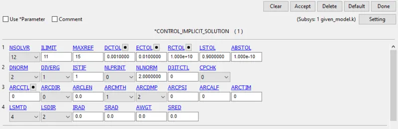
Fig: Control_Implicit_Solution Card 

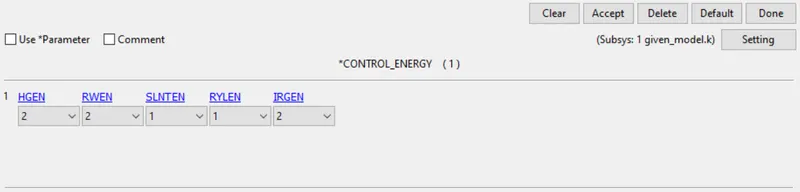
Fig: Control_Energy Card

5.  Results and Discussion:

5.1 MAT_HYPERELASTIC_RUBBER_H Data Comparison

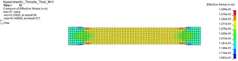
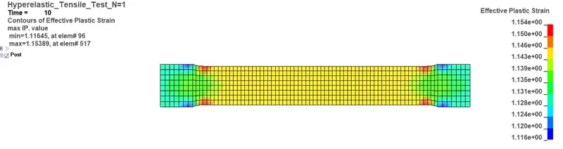
Fig: Effective Stress and Plastic Strain Variation for N=1

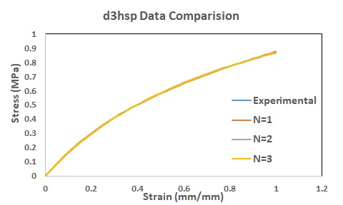
 5.2 Constants obtained from d2hsp file

For N=1;

Mooney	constant	c1	1.77E-01
Mooney	constant	c2	1.47E-01

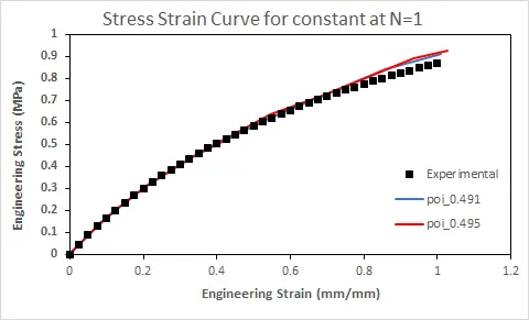
Eng. Stress - Eng. Strain data comparison

For N=2;

Hyperelastic	Constant	C10	2.60E-01
Hyperelastic	Constant	C01	4.59E-02
Hyperelastic	Constant	C11	-2.09E-02
Hyperelastic	Constant	C20	2.91E-03
Hyperelastic	Constant	C02	1.02E-03
Hyperelastic	Constant	C30	0.00E+00

Eng. Stress - Eng. Strain data comparison

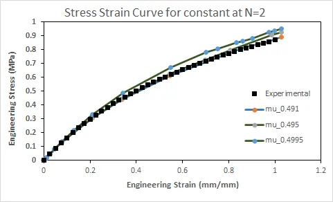
From the analysis, it was determined that the value of the constant in MAT_HYPERELASTIC_RUBBER_H with poison's ratio of 0.491 gave the best fit results. 

For N=3;

Hyperelastic	Constant	C10	2.61E-01
Hyperelastic	Constant	C01	4.42E-02
Hyperelastic	Constant	C11	-6.07E-03
Hyperelastic	Constant	C20	-2.67E-03
Hyperelastic	Constant	C02	-9.97E-03
Hyperelastic	Constant	C30	1.57E-04

Eng. Stress - Eng. Strain data comparison

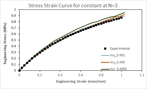
As obtained in the previous simulations, the same trend was observed where the stress-strain curve was more close to the experimental curve when the Poisson's ratio was about 0.491. 

5.1 MAT_OGDEN_RUBBER_O Data Comparison

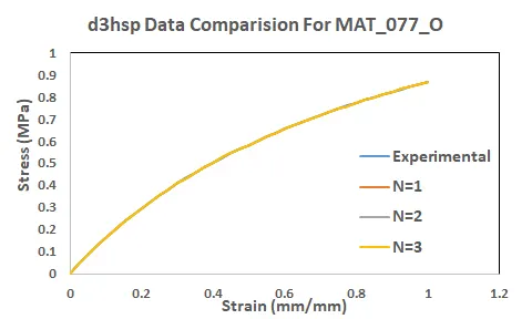
Fig: Effective Stress and Plastic Strain Variation for N=1

 5.2 Constants obtained from d2hsp file

For N=1;

mu(1)=	9.11E-01
alpha(1)=	1.34E+00

Eng. Stress - Eng. Strain data comparison 

For N=2;

mu(1)	9.16E-01
alpha(1)	1.34E+00
mu(2)	2.23E+00
alpha(2)	-1.84E-03

Eng. Stress - Eng. Strain data comparison

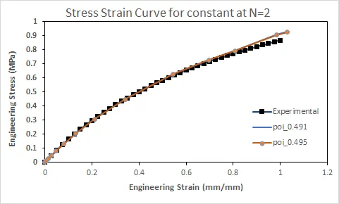
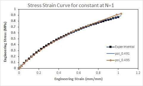
From the analysis, it was determined that the value of the constant in MAT_OGDEN_RUBBER_O with poison's ratio of 0.491 gave the best fit results. 

For N=3;

mu(1)	-3.18E-02
alpha(1)	1.93E+00
mu(2)	2.61E-01
alpha(2)	1.55E+00
mu(3)	6.82E-01
alpha(3)	1.29E+00

Eng. Stress - Eng. Strain data comparison

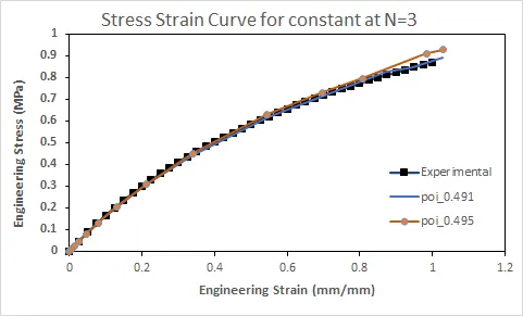
As obtained in the previous simulations, the same trend was observed where the stress-strain curve was more close to the experimental curve when the Poisson's ratio was about 0.491. 

CONCLUSION

•  Two material models have been utilised to simulate the tensile test of a hyperelastic material model using experimental data. 
• MAT_HYPERELASTIC_RUBBER_H material model was utilised as it provides a general hyperelastic rubber model combined optionally with linear viscoelasticity as outlined by Christensen. 
• Using N=0, hyperelastic constants obtained from the d3hsp file were are input directly and the engineering stress-strain graph was compared with experimental data.
  C10 𝐶10
  C01 𝐶01
  C11 𝐶11
  C20 𝐶20
  C02 𝐶02
  C30 𝐶30
• N=1,2,3 were utilised and it was determined that N=1 with poisons ratio =0.491 gave the best fit result. 
• MAT_MAT_OGDEN_RUBBER_O material model was utilised as this material model provides the Ogden rubber model combined optionally with linear viscoelasticity given by Christensen.
• Using N=0, hyperelastic constants obtained from the d3hsp file were are input directly and the engineering stress-strain graph was compared with experimental data. The constants were obtained in the form of MUi 𝜇𝑖 and ALPHAi 𝛼𝑖. Both the constants can carry up to 8 but only up to 3 variables were utilised for this study.
• Similar to the MAT_HYPERELASTIC_RUBBER_H material model, MAT_MAT_OGDEN_RUBBER_O showed similar results where N=1 with poisons ratio =0.491 gave the best fit result.