Week - 10 Hyperelastic Material Models

Hyperelastic Material Modelling

Objective

To compare data from the given engineering stress vs engineering strain for a hyperelastic material to the fitted data.

Condition

- Vary the constant n=1,233 for hyperelastic and Ogden material model.

- The units system to be used is kg-mm-ms

Theory

The hyperelastic material model:

• is isotropic and nonlinear;
• is valid for materials that exhibit instantaneous elastic response up to large strains (such as rubber, solid propellant, or other elastomeric materials); and
• requires that geometric nonlinearity be accounted for during the analysis step since it is intended for finite-strain applications.

Hyperelastic materials are described in terms of a “strain energy potential,” , which defines the strain energy stored in the material per unit of reference volume (volume in the initial configuration) as a function of the strain at that point in the material. There are several forms of strain energy potentials available in Ls dyna to model approximately incompressible isotropic elastomers: the Arruda-Boyce form, the Marlow form, the Mooney-Rivlin form, the neo-Hookean form, the Ogden form, the polynomial form, the reduced polynomial form, the Yeoh form, and the Van der Waals form. As will be pointed out below, the reduced polynomial and Mooney-Rivlin models can be viewed as particular cases of the polynomial model; the Yeoh and neo-Hookean potentials, in turn, can be viewed as special cases of the reduced polynomial model. Thus, we will occasionally refer collectively to these models as “polynomial models.”

Generally, when data from multiple experimental tests are available (typically, this requires at least uniaxial and equibiaxial test data), the Ogden and Van der Waals forms are more accurate in fitting experimental results. If limited test data are available for calibration, the Arruda-Boyce, Van der Waals, Yeoh, or reduced polynomial forms provide reasonable behaviour. When only one set of test data (uniaxial, equibiaxial, or planar test data) is available, the Marlow form is recommended. In this case, a strain energy potential is constructed that will reproduce the test data exactly and that will have reasonable behaviour in other deformation modes.

True strain = ln(1 + engineering strain) where ln designates the natural log

True stress = (engineering stress) * exp(true strain) = (engineering stress) * (1 + engineering strain) where exp(true strain) is 2.71 raised to the power of (true strain).

Effective Plastic Strain = Strain –

E=Youngs Modulus

Procedure

• Add the values of stress and strain in an excel sheet.

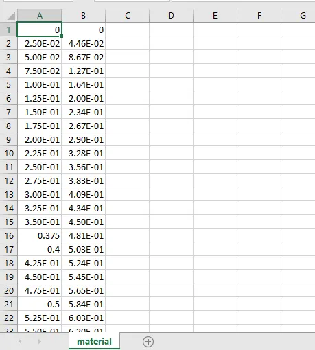
• Save the file as a .CSV format.
• After Importing the keyword file, we can start by creating the section shell card.

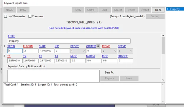
• Define the curve for material data.

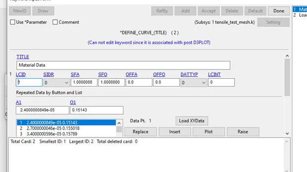
• Load X/Y data and select the .csv file created previously.

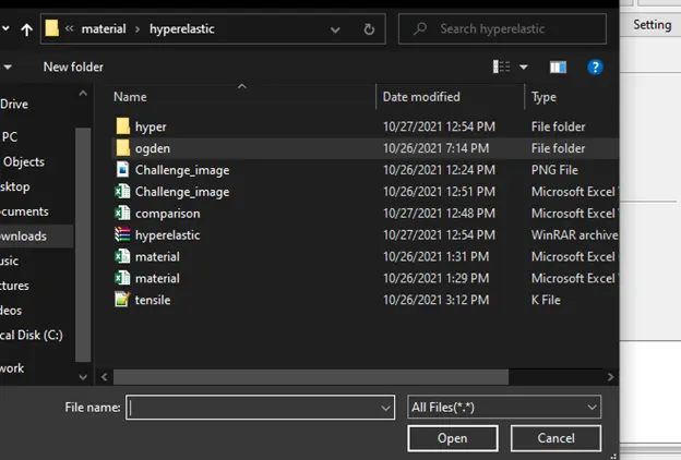
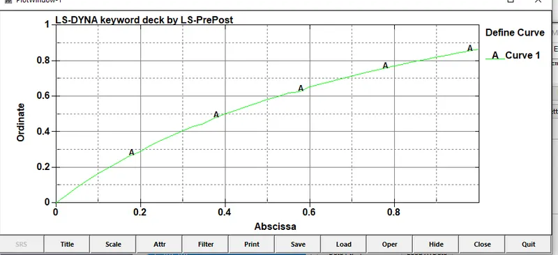
Define the Load Curve

• In keyword manager, go to define curve and plot the values appropriately for a linear increase.

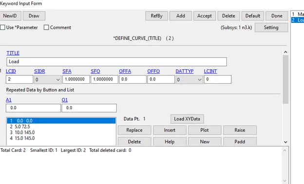
v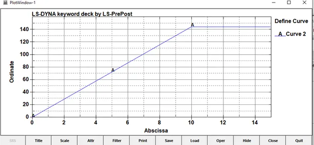

Material Data

• Create a mat77_h and mat77_O card and add the values appropriately.

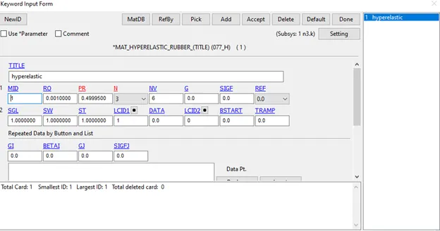
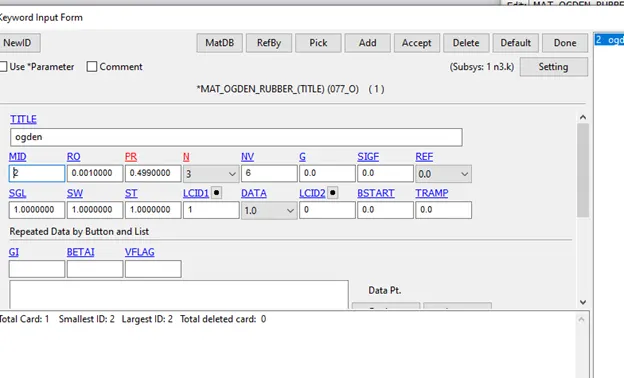
Note: for Ogden, change the value of N to 3 to see the LCID option.

Boundary Conditions

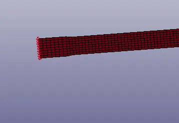
• Set the final layer of nodes on one side of the model as rigid on the x axis.

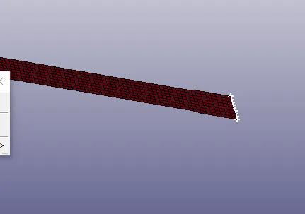
• For better stability, set the centre nodes of both side rigid on the y axis

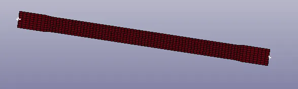
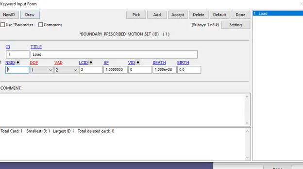
• After this,create a prescribed motion set for displacement.Set only the last layer of nodes opposite to the rigid ones for the Node Set Id

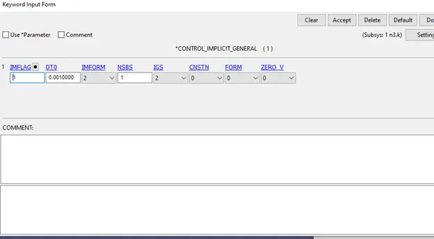
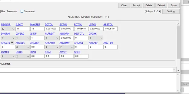
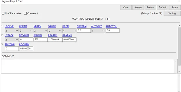
• Since the loading can be considered as Quasi Static , implicit solver can be chosen for this simulation and as such, implicit control keycards need to be created.
• It is recommended to go with the default properties for now
• 

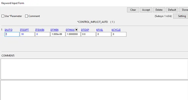
Set IAuto to 1 as you get convergence error during the simulation otherwise.

Output Files

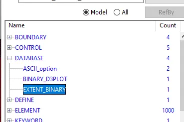
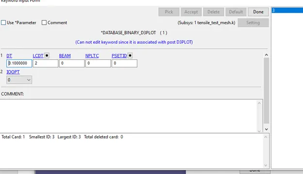
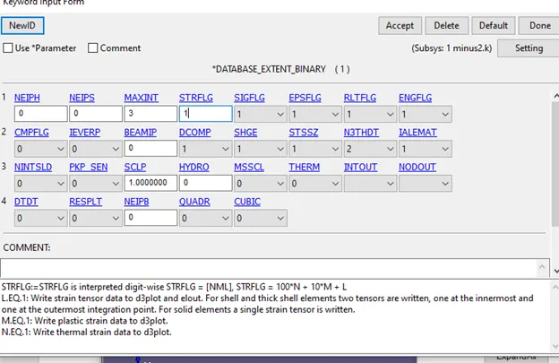
• In database, create the d3plot,extent binary and Ascii keywords

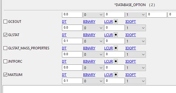
• In Ascii,enable Glstat and Matsum.

In extent Binary,set the values appropriately.

Control

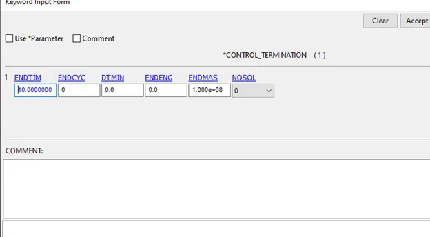
• Create a Control Termination Keyword

Check the keywords using the model checker for errors

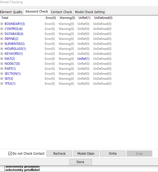
No errors only unref for the material card cases.

After this run the simulation using the ls dyna solver

Make sure that the folder has no spaces and the termination is normal termination.

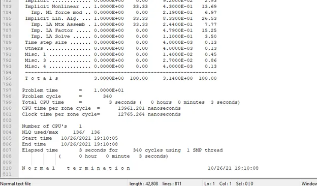
Repeat the same by varying the value of n from 1-3 for hyperelastic and ogden material model.

Post Processing

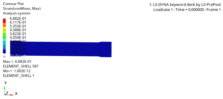
Since, we are using a hyper elastic material there is no failure despite high strain

In the d3hsp file, find the fitted data.

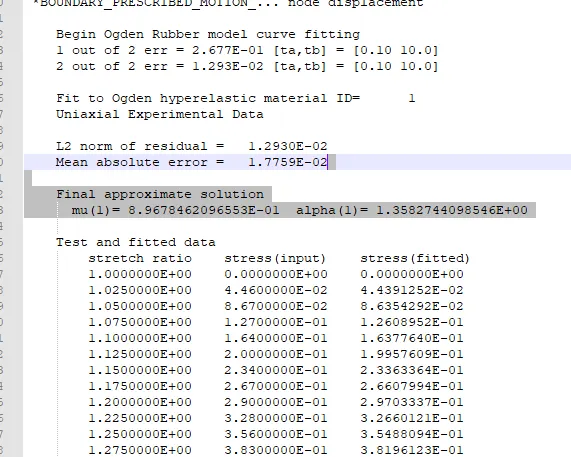
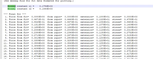
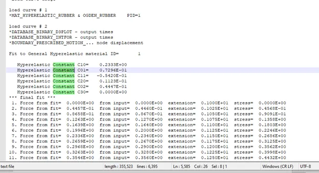
Note in ogden, you get stretch ratio and engineering stress

For hyperelastic, you get stretch ratio and true stress.

Plot them using excel.

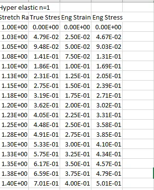
Plot the Stress vs Strain graphs for the material data and simulation data.

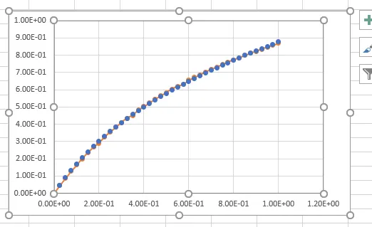
After plotting them ,it can be observed that the graphs are perfectly collinear, indicating a good fit for the material behaviour.

Similarly compare the graphs for the various other cases.

Case 1:
Hyperelastic, n=1

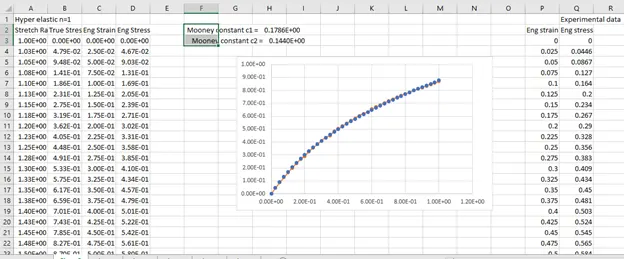
Mooney constant c1 = 0.1786E+00

Mooney constant c2 = 0.1440E+00

Case 2:

Hyperelastic n=2

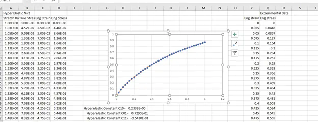
Hyperelastic Constant C10= 0.2333E+00

Hyperelastic Constant C01= 0.7296E-01

Hyperelastic Constant C11= -0.5420E-01

Hyperelastic Constant C20= 0.1123E-01

Hyperelastic Constant C02= 0.4447E-01

Hyperelastic Constant C30= 0.0000E+00

Case3: Hyperelastic N=3

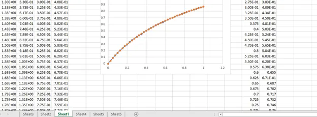
Hyperelastic Constant C10= 0.1697E+00

Hyperelastic Constant C01= 0.1401E+00

Hyperelastic Constant C11= -0.6261E+00

Hyperelastic Constant C20= 0.2262E+00

Hyperelastic Constant C02= 0.4677E+00

Hyperelastic Constant C30= -0.6030E-02

Case 4:
Ogden n=1

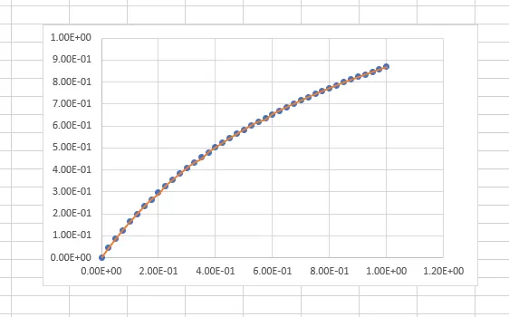
Final approximate solution

mu(1)= 8.9678462096553E-01 alpha(1)= 1.3582744098546E+00

Case 5:
Ogden n=2

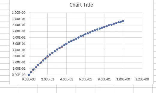
Final approximate solution

mu(1)= 1.0047327558079E+00 alpha(1)= 1.2984381994175E+00

mu(2)= 2.4599571132392E+00 alpha(2)=-3.6241031176921E-02

Case 6:
Ogden n=3

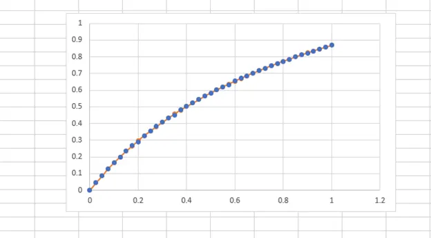
Final approximate solution

mu(1)= 2.1240975823237E+00 alpha(1)= 9.3680151995079E-01

mu(2)= 2.7281216338503E+00 alpha(2)=-5.3795370522187E-01

mu(3)=-4.2090567913795E-01 alpha(3)=-1.6607435197862E+00

It can be noted that the values of stress are more accurate in case 5 and case 6 compared to case 4, higher accuracy can be observed if we include more decimal points in the original material data.

Learning Outcomes

• Implicit Analysis in Ls Dyna
• Cross plotting
• Hyperelastic Material modelling in ls dyna

Conclusion

Material Modelling is an extremely important aspect of modelling an Fea simulation.

In this project, we modelled a hyperelastic material model for a tensile test of a dogbone specimen for 100% strain.After plotting the stress-strain graph , it can be observed that the stress-strain graph is more accurate for the values of n=2,3 for both hyperelastic and ogden material model.

However, there is no significant difference in either hyperelastic77 or ogden material model for the given material data, that is both material models are a good fit for the given material.It should be noted that the ogden model has a higher polynomial degree of upto N=8 compared to the hyperelastic model that has a polynomial limit of N=3.This implies that, ogden material model can more accurately define complex hyperelastic material but at a higher computational cost.