Week - 10 Hyperelastic Material Models

AIM: Calculate the Mooney Rivlin and Ogden material constants and compare the both using stress-strain data from a Dogbone specimen tensile test with 100 percent strain.

PROCEDURE:

• Now we have given a stress and strain for the curve.

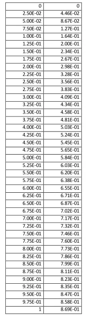
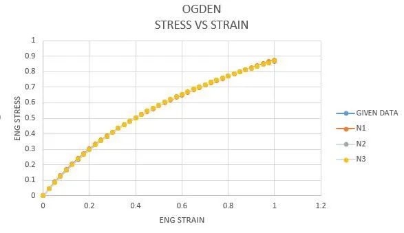
• With the help of this we will plot a cuve in excel.

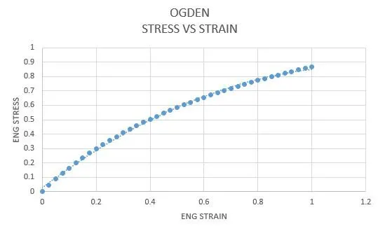
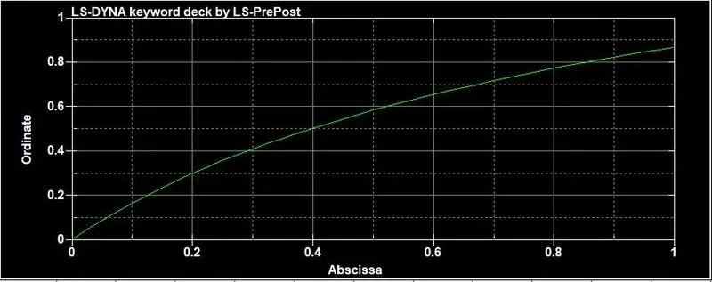
• Now we will open the TENSILE MATERIAL MODEL and insert the given curve points.

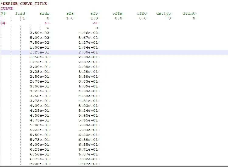
• PLOTTED CURVE:

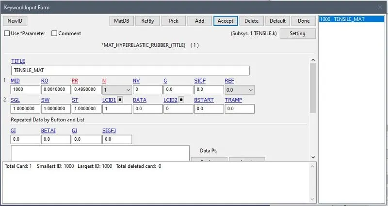
• Now for the material we will choose MAT_HYPERELASTCI_RUBBER_077 and add the the material properties for it.

• For shell section :

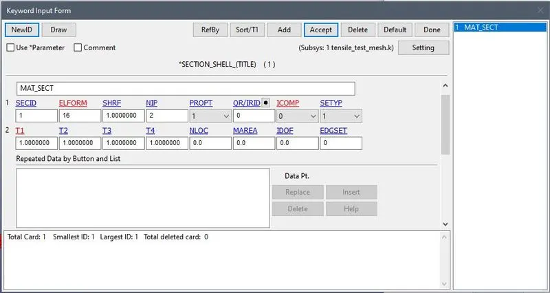
• Now after that we will assign this to the part.
• Once it is done then give the boundary condition to the MODEL.

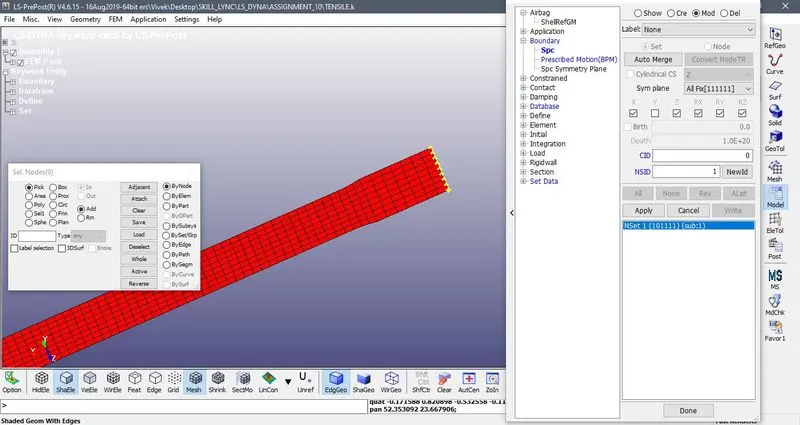
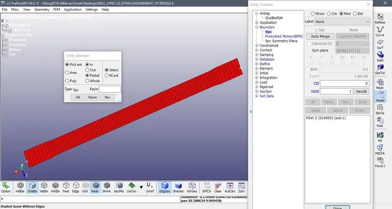
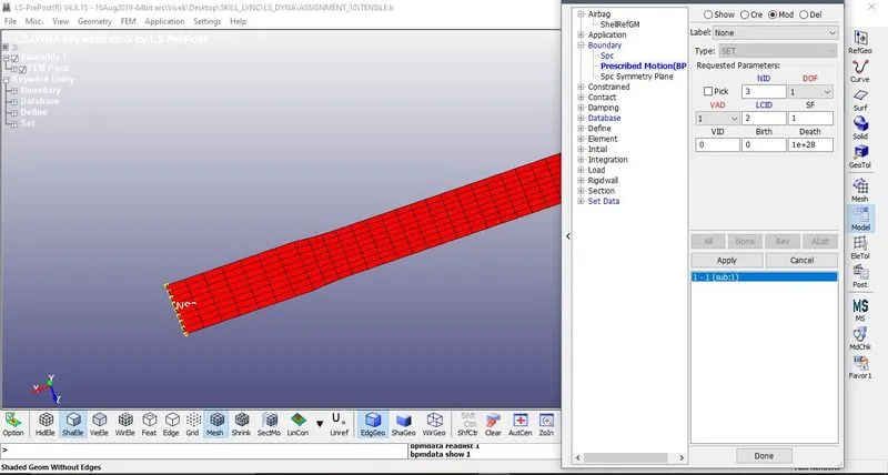
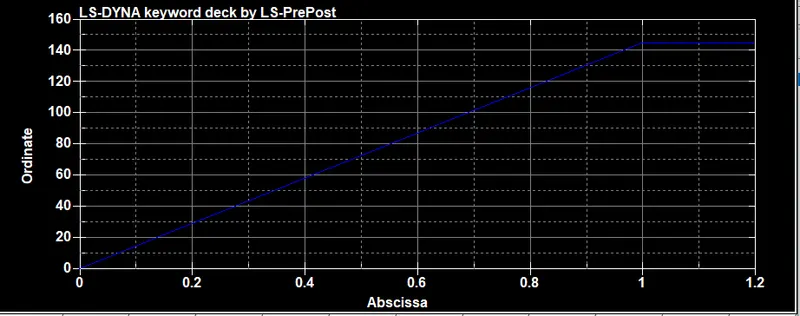
• Since it is mentioned Dogbone specimen tensile test with 100 percent strain, and as the length of the speciemen was 45 mm so the displacement curve as shown below to 145 mm.

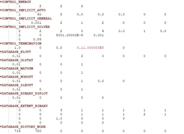
• Now after that give the DATABASE , CONTROL and TERMINATION

• Now after the termination we will open the d3hsp file to find the value of C10 and C01

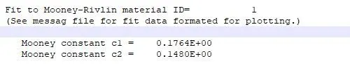
• Now for the other constant we will change the value of N from the MATERIAL card.
• The obtained values are shown below:

N=1

Mooney constant c1 = 0.1764E+00

Mooney constant c2 = 0.1480E+00

N=2

Hyperelastic Constant C10= 0.2794E+00

Hyperelastic Constant C01= 0.2476E-01

Hyperelastic Constant C11= 0.2552E-01

Hyperelastic Constant C20= -0.1008E-01

Hyperelastic Constant C02= -0.4864E-01

Hyperelastic Constant C30= 0.0000E+00

N=3

Hyperelastic Constant C10= 0.2736E+00

Hyperelastic Constant C01= 0.3089E-01

Hyperelastic Constant C11= -0.2670E-01

Hyperelastic Constant C20= 0.9555E-02

Hyperelastic Constant C02= -0.1000E-01

Hyperelastic Constant C30= -0.5506E-03

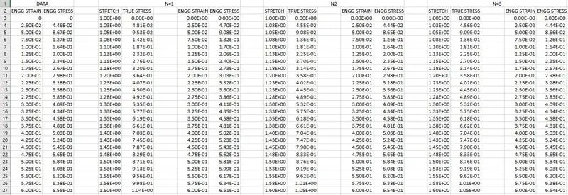
• This way all the values have been converted for all the N1, N2 and N3 value of True stress and stretch to Engineering stress-strain respectively and plotted as a graph for Engineering stress vs Engineering strain.
• DATA:

CURVE:

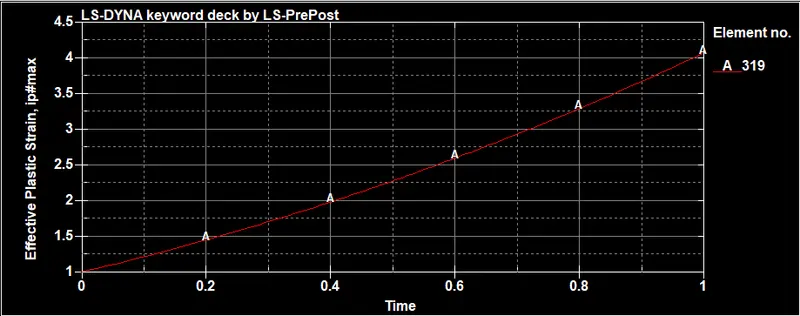
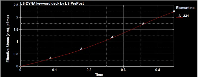
• Now we will put the Mooney Rivlin Constant in the material card and run the simulation. And plot the graphs with the help of those values.

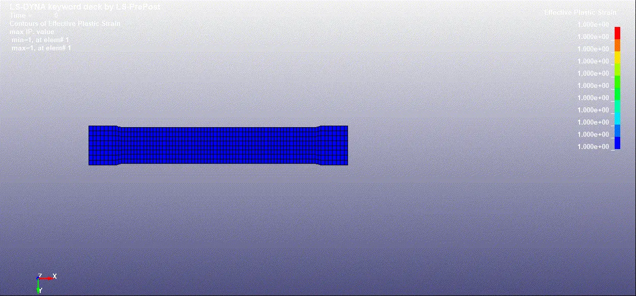
D3PLOT

GRAPH

FOR N=1

1.

2.

.

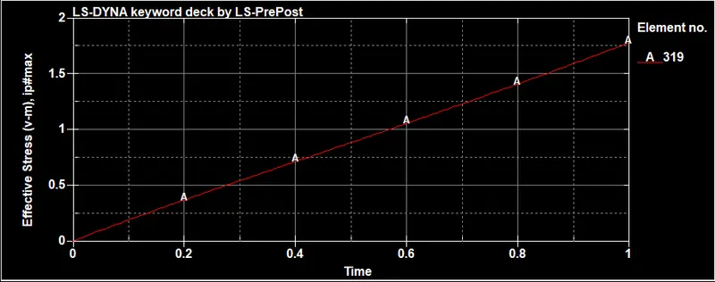FOR N=2

1.

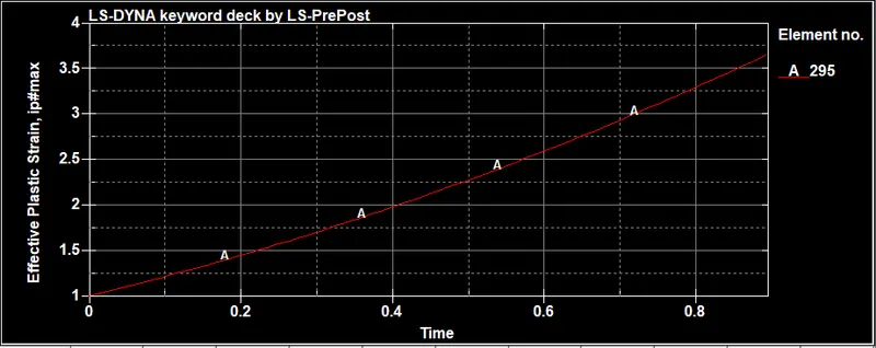
2.

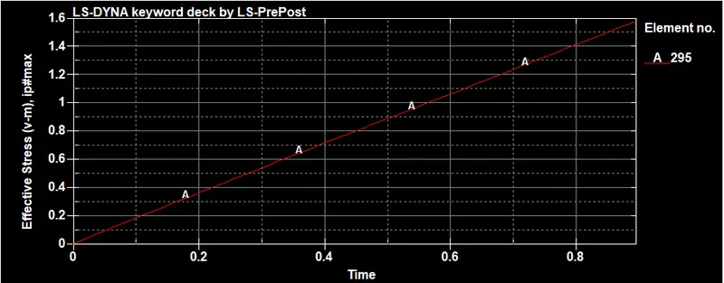
N=3

1.

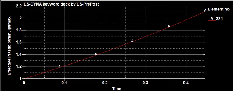
2.

• Now Next we will create a OGDEN MATERIAL and follow the same process.

N=1			N=5
mu(1)= 9.1322000486764E-01	alpha(1)= 1.3398691179143E+00		mu(1)=-3.1312241691562E+01	alpha(1)=-5.2357360108085E-01
			mu(2)= 2.7152807056193E+01	alpha(2)=-1.9857168137085E+00
			mu(3)=-2.1657204150715E+01	alpha(3)=-3.3136165481104E+00
N=2			mu(4)= 9.3456820669476E+00	alpha(4)=-4.6955706973702E+00
mu(1)= 9.1262801457576E-01	alpha(1)= 1.3402097351283E+00		mu(5)=-1.8311538721810E+00	alpha(5)=-5.9286042684786E+00
mu(2)= 2.3107742942407E+00	alpha(2)= 2.1482469257717E-04
			N=6
			mu(1)=-4.4795390914825E+00	alpha(1)= 2.3704245886910E+00
			mu(2)= 7.8891950235611E+01	alpha(2)= 7.8984736377231E-01
			mu(3)= 1.8664437232080E+02	alpha(3)=-7.8129254626863E-01
			mu(4)=-7.7446639870649E+01	alpha(4)=-2.3904894464536E+00
N=3			mu(5)= 3.0182620925577E+01	alpha(5)=-3.9612477762752E+00
mu(1)= 1.4503785325353E+00	alpha(1)= 1.1253306481408E+00		mu(6)=-5.2732859882963E+00	alpha(6)=-5.6479785726203E+00
mu(2)= 2.9910476212275E+00	alpha(2)=-3.4716039406001E-01
mu(3)=-6.2502806327930E-01	alpha(3)=-1.0114623967499E+00		N=7
			mu(1)=-7.4238721222157E+00	alpha(1)= 2.2499391010117E+00
			mu(2)= 1.2727172549007E+02	alpha(2)= 7.4997778151728E-01
			mu(3)= 2.9658388531461E+02	alpha(3)=-7.4999685939963E-01
			mu(4)=-1.1983195066990E+02	alpha(4)=-2.2500326574150E+00
N=4			mu(5)= 4.2920915985735E+01	alpha(5)=-3.7503378106777E+00
mu(1)= 1.5899020863525E-01	alpha(1)= 1.8720418326878E+00		mu(6)=-6.0285213146379E+00	alpha(6)=-5.2516141413689E+00
mu(2)= 1.8064766613912E+00	alpha(2)= 7.7760137610344E-01		mu(7)=-6.8234814651144E-01	alpha(7)=-6.7451525405687E+00
mu(3)= 1.3495946801348E+00	alpha(3)=-6.0335316085203E-01
mu(4)=-2.0514708712778E-01	alpha(4)=-1.6421541516334E+00		N=8
			mu(1)= 2.5367490326143E+02	alpha(1)=-7.2357952789485E-01
			mu(2)=-5.5821969634356E+02	alpha(2)=-2.2422670297489E+00
			mu(3)= 9.5435318431782E+02	alpha(3)=-3.7441848897163E+00
			mu(4)=-1.0698301521183E+03	alpha(4)=-5.2474686310127E+00
			mu(5)= 7.7347073049968E+02	alpha(5)=-6.7500840885322E+00
			mu(6)=-3.4548065951316E+02	alpha(6)=-8.2524061419601E+00
			mu(7)= 8.6175936095479E+01	alpha(7)=-9.7541535614775E+00
			mu(8)=-9.1509608465285E+00	alpha(8)=-1.1255720749196E+01

CONCLUSION:

• The Mooney-Rivlin and Ogden material constants are obtained from d3hsp file by inputting the value of polynomial N=1,2,3 in the material card MAT_77_H and MAT_77_O.
• The Ogden material model has more polynomials ranging from 1 to 8 and is easy to use and gives better adjustment to experimental data at the cost of computional time.
• The required graphs are plotted.