Hyperelastic Material Modelling using LS-DYNA

AIM:

1. To calculate the Mooney Rivlin and Ogden material constants and compare the both using stress-strain data from a Dogbone specimen tensile test with 100 percent strain.
2. The given material data is the engineering stress-strain in MPa/(mm/mm).
3. The comparison should be shown from the d3hsp file and using simulation.

Note: The unit system used is g-mm-ms, N, MPa, N-mm.

PROCEDURE:

Analysis setup for Material model verification:

1. Experimental Data:

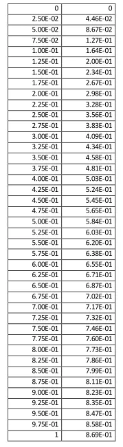
Fig.1 Experimental data of Engg. stress and Engg. strain of hyperelastic material.

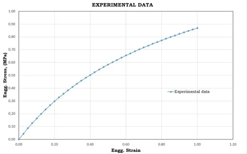
Fig.2 Experimental data plotted with Engg. stress vs Engg. strain.

The given data of Engg. stress and Engg. strain of hyperelastic material is plotted in excel is as shown in fig.2.

2. Hyperelastic Material Model:

Hyperelastic constitutive models describe the elastic property of a material from the strain energy. The specific form of the strain energy controls the elastic material properties of the model. There are many different kinds of functions. They all try to follow the stress stretch curve for different loading cases. The simplest ones are built as a polynomial.

The given material data refers to rubber which is generally considered to be fully incompressible since the bulk modulus greatly exceeds the shear modulus in magnitude. To model the rubber as an unconstrained material a hydrostatic work term, 𝑊_H(𝐽), is included in the strain energy functional which is function of the relative volume, 𝐽. They are usually written in the following form,

`W(J_1,J_2,J)=∑_(p,q=0)^nC_(pq) (J_1-3)^p (J_2-3)^q+W_H (J)`

i) The Mooney-Rivlin rubber model is obtained by specifying 𝑛 = 1.

`W=C_10 (I_1-3)+C_01 (I_2-3)`

where, C₁₀ and C₀₁ are Mooney-Rivlin constants. MAT_77_H material card is used to find these constants and obtain a curve matching with experimental data.

ii) The Ogden rubber model is obtained from the equation,

`W(λ_1,λ_2,λ_3 )=∑_(p=1)^nμ_p/α_p (λ_1^(α_p )+λ_2^(α_p )+λ_3^(α_p )-3)`

Where, `μ_p` and `α_p` are Ogden constants. MAT_77_O material card is used to find these constants and obtain a curve matching with experimental data.

3. Part definition:

To verify and validate the given material data with material models of Mooney-Rivlin and Ogden a dogbone specimen is taken for the analysis.

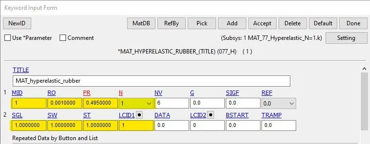
Fig.3 Material card for hyperelastic rubber model with N=1

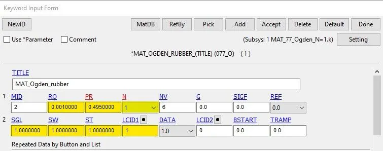
Fig.4 Material card for Ogden rubber model with N=1

To find the Mooney-Rivlin and Ogden constants the value of N is set to 1. The value of density and Poisson’s ratio are taken as generic value for the rubber material.

For N>0, data from a uniaxial test are used.

SGL Specimen gauge length

SW Specimen width

ST Specimen thickness

The value of SGL, SW, and ST are set to unity (1.0), then the curve LCID1 is engineering stress versus engineering strain as shown in fig. 5.

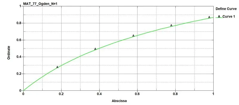
Fig.5 LCID1 curve for given data of Engg. stress vs Engg. strain.

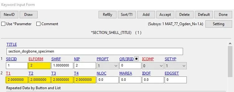
Fig.6 Section property of dogbone specimen.

The section property of dogbone specimen is assigned as shell element with 2 mm thickness and ELFORM=2.

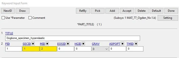
Fig.7 Part definition of dogbone specimen.

4. Boundary Condition:

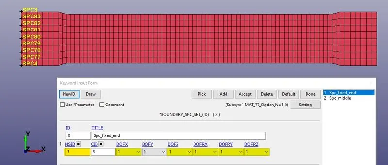
Fig.8 The nodes at the fixed end constrained in X and Z direction.

The nodes at the fixed end is constrained in X and Z direction only and Y direction is not constrained because of lateral expansion during tensile test.

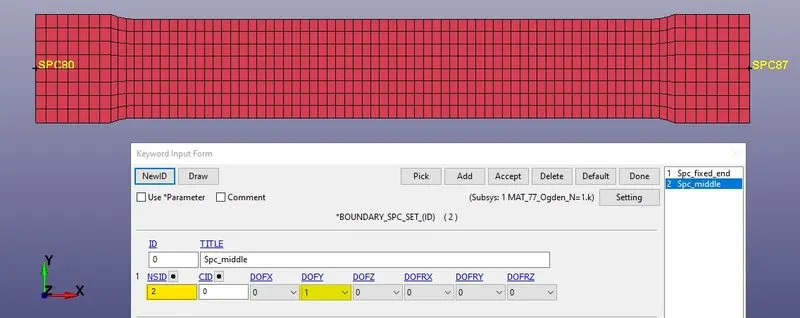
Fig.9 The nodes at the middle constrained in Y direction.

The nodes at the middle is constrained in Y direction since the neutral axis passes through the middle of the specimen in X direction.

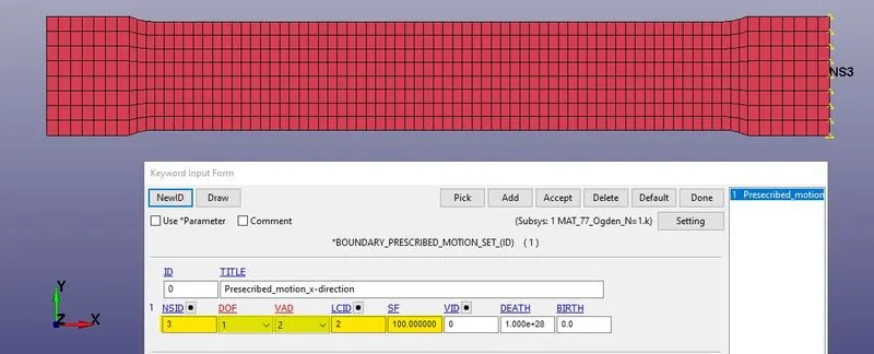
Fig.10.1 Boundary prescribed motion in the pulling end of specimen.

The nodes of the pulling end are assigned with a boundary prescribed motion in X direction using displacement load curve LCID as shown in fig. 10.2.

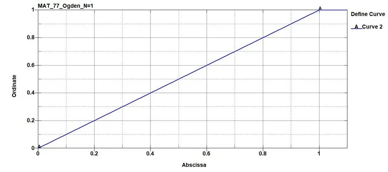
Fig.10.2 Displacement load curve.

5. Control Functions:

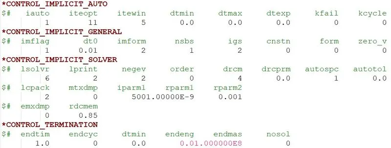
Fig.11 Control functions for implicit analysis.

The tensile test of given dogbone specimen is considered as quasi-static analysis, hence implicit analysis is carried out with necessary control implicit cards as shown in fig.11. The keyword file is saved and made to run in LS-DYNA program manager to get d3hsp file.

Note: The keyword file for each material model is set up separately and made to run individually.

II. Analysis setup for Material model validation:

The d3hsp file for each material model is opened in notepad++ and the material constants of Mooney-Rivlin and Ogden as well as final fit data of stretch and Engg. stress is obtained for each case.

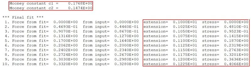
Fig.12 d3hsp file of Mooney-Rivlin material model.

From the output files of material verification, d3hsp file is opened in notepad++ as shown in fig. 12. The Mooney-Rivlin constants obtained are

C₁₀ = c1 = 0.1768E+00

C₀₁ = c2 = 0.1474E+00

For material model validation, the value of N is changed to 0 in the material card. These values are inputted to the material card MAT_77_H as shown in fig. 13. The data obtained from d3hsp file is extension (stretch) and True stress which is converted to Engg. strain and Engg, stress to verify with experimental data.

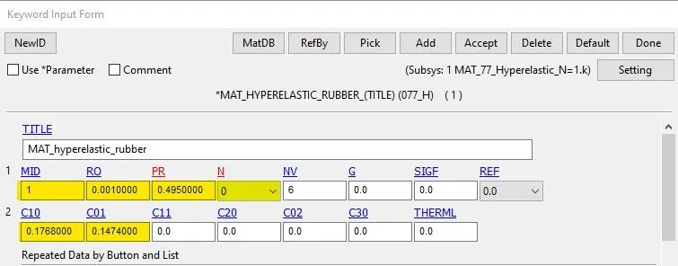
Fig.13 Material card for hyperelastic rubber model with N=0

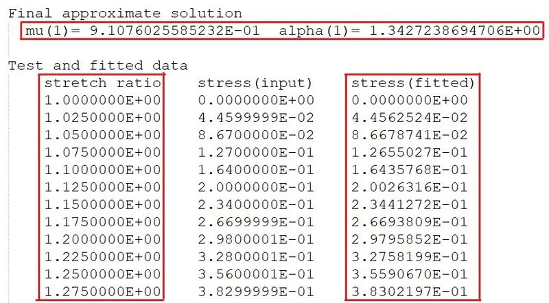
Fig.14 d3hsp file of Ogden material model.

From the d3hsp output file of Ogden material model the Ogden constants obtained are

`μ_1=9.1076025585232E-01`

`α_1=1.3427238694706E+00`

These values are inputted to the material card MAT_77_O as shown in fig. 15. The data obtained from d3hsp file is Engg. Stress and stretch ratio which is converted to Engg. strain to verify with experimental data.

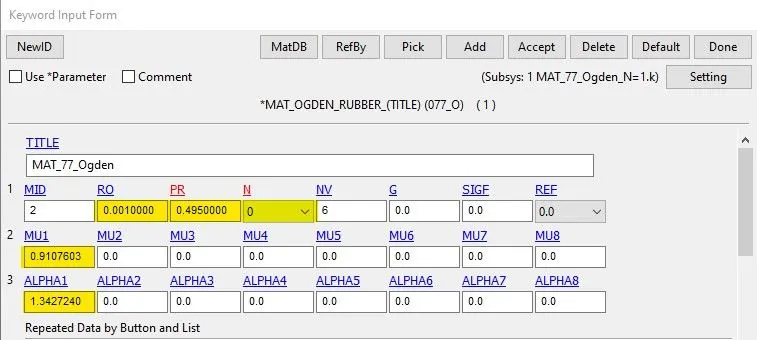
Fig.15 Material card for Ogden rubber model with N=0

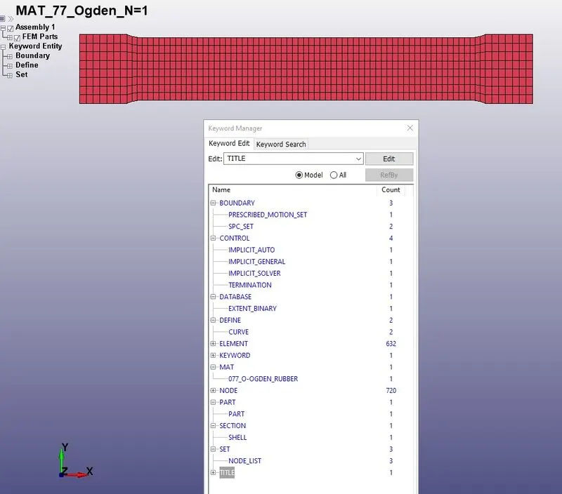
Fig.16 Keywords used for the simulation of material validation.

The keywords used for material model validation is same as that of material model verification except the changes to material card(N=0) and addition of database extent binary to compute elastic strain is as shown in fig.16. The keyword file is saved and made to run in LS-DYNA program manager to get requested output file.

Note: The simulation is carried out for different polynomial values of N=1,2,3 for each material model so as to get better adjustment to the experimental results.

RESULTS AND DISCUSSIONS:

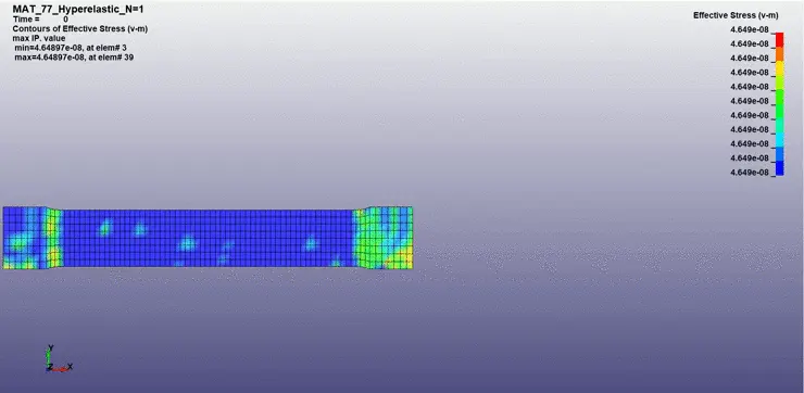
1. The animation of Von-Mises stress contour.

i) Mooney-Rivlin material model:

ii) Ogden material model:

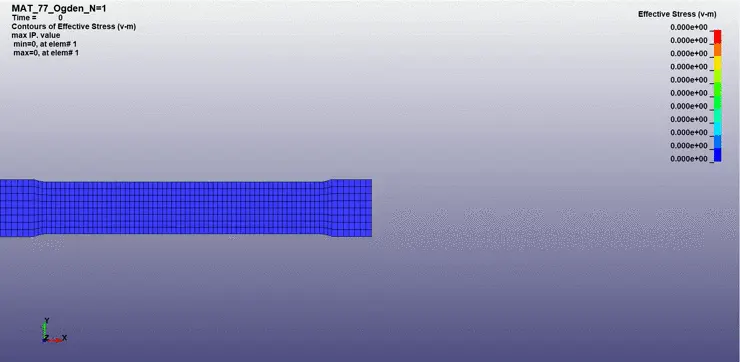
The maximum value of v-m stress developed for Mooney-Rivlin material model(N=1) is 1.66801 MPa, whereas for Ogden material model(N=1) maximum v-m stress is equal to 1.65691 MPa. Hence, the maximum v-m stress value developed is equal for both the material model.

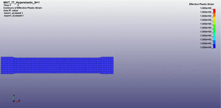
2. The animation of Effective Plastic Strain contour.

i) Mooney-Rivlin material model:

ii) Ogden material model:

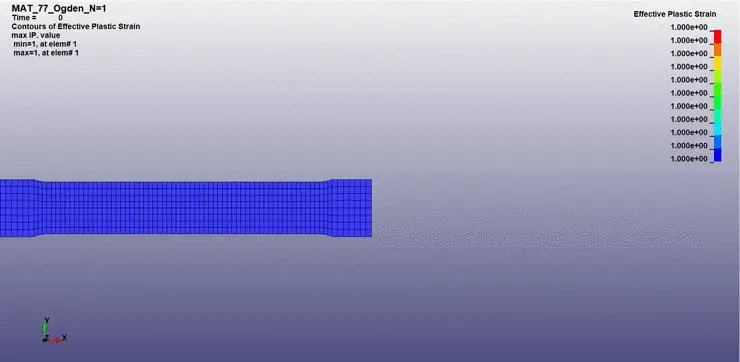
The maximum Effective plastic strain developed for both material models is equal to 3.8.

3. Material model verification:

i) Mooney-Rivlin material model:

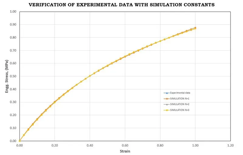
Fig.17 Plot of simulation results of constants verification with experimental data.

ii) Ogden material model:

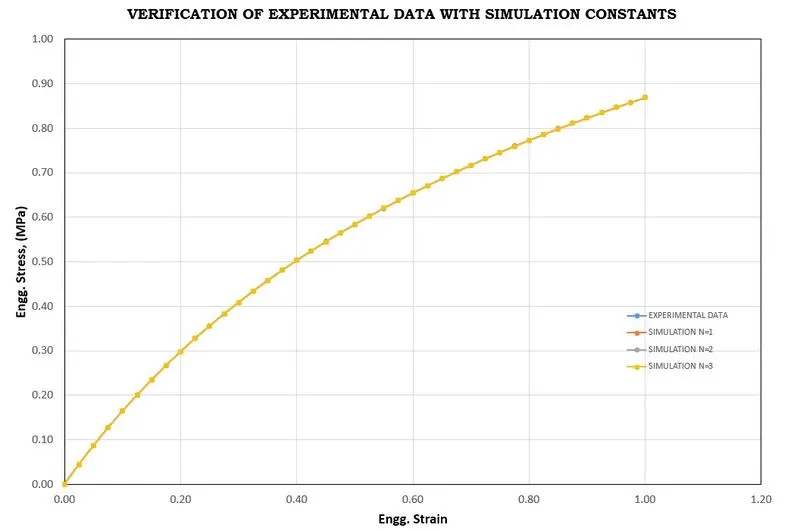
Fig.18 Plot of simulation results of constants verification with experimental data.

From the data obtained from d3hsp file for different polynomial values i.e, (N=1,2,3) curves are plotted with Engg. stress vs Engg. strain in excel with comparison to Experimental data is as shown in fig.17 and Fig.18. It is observed from the graph, that the curves for different polynomial are superimposing and is better adjusted with the experimental data. The Ogden material model gives close fit compared to Mooney-Rivlin material model.

4. Material model validation:

i) Mooney-Rivlin material model:

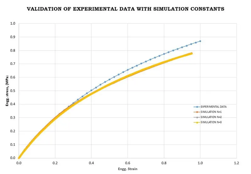
Fig.19 Plot of simulation results of constants validation with experimental data.

ii) Ogden material model:

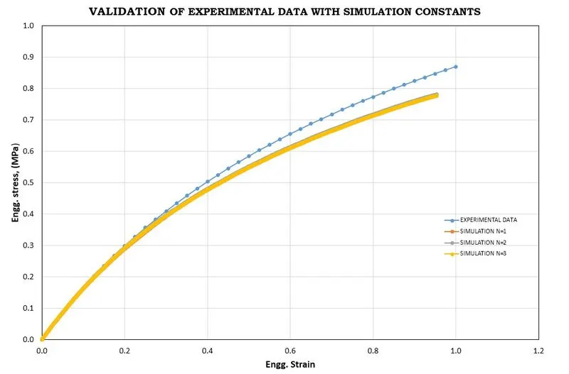
Fig.20 Plot of simulation results of constants validation with experimental data.

For validation, the plot of true stress vs true strain for a middle element of dogbone specimen is saved in .csv file format. The file is opened in excel and the values of true stress and strain are converted to Engg. stress and Engg. strain to plot the curves as shown in fig.19 and Fig. 20. Form the graph, there is a slight deviation of simulation results compared to experimental data for both the material models because the material is highly non-linear and generic values of density and Poisson’s ratio was considered for simulation.

5. Comparison of Mooney-Rivlin and Ogden material model:

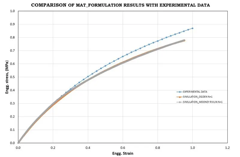
Fig.21 Plot of validation results of Mooney-Rivlin and Ogden constants with experimental data.

From the graph, both material models are behaving similar for the given material data. The Ogden material model has polynomials ranging from 1 to 8 and is easy to use and gives better adjustment to experimental data.

CONCLUSION:

1. The Mooney-Rivlin and Ogden material constants are obtained from d3hsp file by inputting the value of polynomial N=1 in the material card MAT_77_H and MAT_77_O
2. The stretch stress curve data obtained from d3hsp for both hyperelastic constitutive models were verified with experimental material data and found to be a close fit.
3. The simulation results of tensile test for both material models with experimental data showed a slight deviation due to high non-linear behaviour of the given hyperelastic material and the generic values of density and Poisson’s ratio.
4. From the simulation results, both hyperelastic constitutive material models were found to be valid to describe the behaviour of the given material data.
5. The Ogden material model has more polynomials ranging from 1 to 8 and is easy to use and gives better adjustment to experimental data at the cost of computional time.
6. Learned to verify and validate hyperelastic material model for the given material data.

Google Drive Link:Hyperelastic Material modelling using LS-DYNA