Week - 10 Hyperelastic Material Models

Hyperelastic Material Models

OBJECTIVE:-

1. To calculate and compare the Mooney Rivlin, Ogden material constants using stress-strain data by 100 percent strain.
2. From the above condition simulate and validate the material model using MPa(mm/ms).
3. Finally, compare the d3hsp file from the simulation.

INTRODUCTION:-

Hyperelastic materials are the special class of materials that respond elastically even when they are subjected to large deformations. They show both a nonlinear material behavior as well as large shape changes. They are characterized by-

1. Can undergo large elastic deformations in order of 100 to 700% which are fully recoverable, i.e., the initial shape is recovered when the load is removed.
2. Are nearly incompressible, which means that they change can their shape but overall volume remains almost constant.
3. Show a highly nonlinear stress-strain relation.
4. The material softens and then becomes stiffer again when applied to tension whereas, under compression, they have a quite stiff response.

Many polymers show hyperelastic behavior, such as elastomers, rubbers, and other similar soft flexible materials.

• Hyperelastic material models are regularly used to represent the large deformation behavior of materials with FEA. They are commonly used to model mechanical behaviors of unfilled/filled elastomers.
• In addition to elastomers, hyperelastic material models are also used to approximate the material behavior of biological tissues, polymeric foams, etc. Linearly elastic materials are described through two material constants (Young’s modulus and Poisson ratio).
• In contrast, hyperelastic materials are described through a strain-energy density function. The strain-energy density can be used to derive a nonlinear constitutive model (i.e., stresses as a function of large strain deformation measures like deformation)
• Those are derived by researches and some acceptable models we are using popularly such as-
  Ogden
  Neo-Hookean
  Arruda-Boyce
  Yeoh and Fleming
  Mooney-Rivlin and Signorini models

MOONEY RIVLIN:

The strain energy density function for an incompressible Mooney–Rivlin material is defined below. Where ` are empirically determined material constants, I1 and I2 are the first and the second invariant. By varying the Index values of i and j we can change the constitutive equations and use them appropriately for our component. Similarly, we will be having multiple coefficients C
This changing of the index will be basically changing the order of the polynomial of the energy density equation. We need to find out the coefficients of these material models for a different order of the polynomial and extract the best fit curve data from the D3HSp file and compare it with the material curve.

OGDEN MATERIAL:

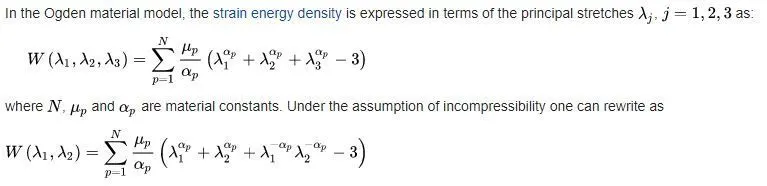
The Ogden material model is a hyperelastic material model used to describe the non-linear stress–strain behavior of complex materials such as rubbers, polymers, and biological tissue. The model was developed by Raymond Ogden in 1972. The Ogden model, like other hyperelastic material models, assumes that the material behavior can be described by means of a strain energy density function, from which the stress–strain relationships can be derived

PROCEDURE:-

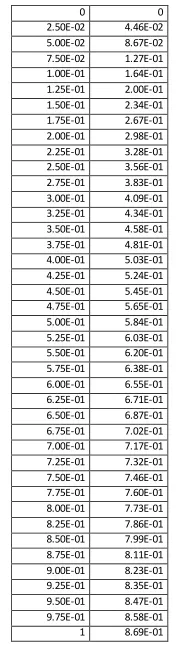
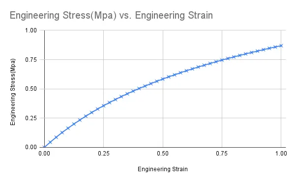
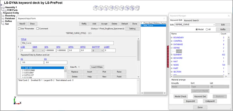
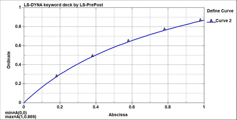
1.The data for the given engineering stress-strain values were arranged and plotted a curve in an excel sheet.

Engineering Strain	Engineering Stress(Mpa)
0	0
2.50E-02	4.46E-02
5.00E-02	8.67E-02
7.50E-02	1.27E-01
1.00E-01	1.64E-01
1.25E-01	2.00E-01
1.50E-01	2.34E-01
1.75E-01	2.67E-01
2.00E-01	2.98E-01
2.25E-01	3.28E-01
2.50E-01	3.56E-01
2.75E-01	3.83E-01
3.00E-01	4.09E-01
3.25E-01	4.34E-01
3.50E-01	4.58E-01
3.75E-01	4.81E-01
4.00E-01	5.03E-01
4.25E-01	5.24E-01
4.50E-01	5.45E-01
4.75E-01	5.65E-01
5.00E-01	5.84E-01
5.25E-01	6.03E-01
5.50E-01	6.20E-01
5.75E-01	6.38E-01
6.00E-01	6.55E-01
6.25E-01	6.71E-01
6.50E-01	6.87E-01
6.75E-01	7.02E-01
7.00E-01	7.17E-01
7.25E-01	7.32E-01
7.50E-01	7.46E-01
7.75E-01	7.60E-01
8.00E-01	7.73E-01
8.25E-01	7.86E-01
8.50E-01	7.99E-01
8.75E-01	8.11E-01
9.00E-01	8.23E-01
9.25E-01	8.35E-01
9.50E-01	8.47E-01
9.75E-01	8.58E-01
1.00E+00	8.69E-01

2.Now the .k file of the given model was opened in the Ls-Pre post.

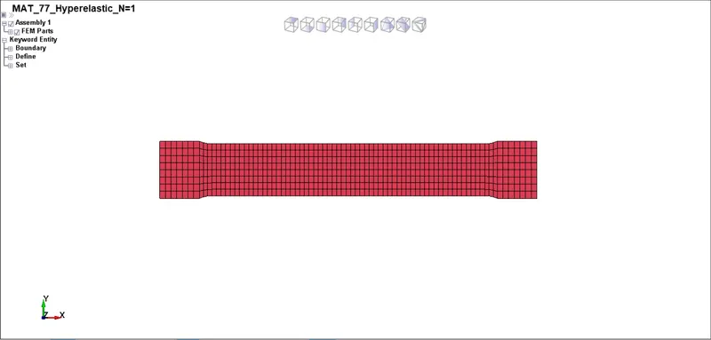
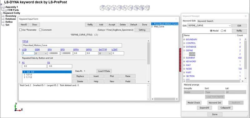
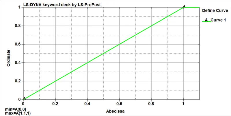
3.Defining Load Curve and Material Curve.

4.Defining Boundary Conditions.

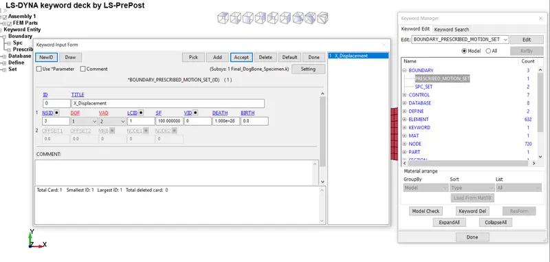
The displacement was given to the end nodes using *BOUNDARY_PRESCRIBED_MOTION_SET. The value for the displacement was calculated as follows.

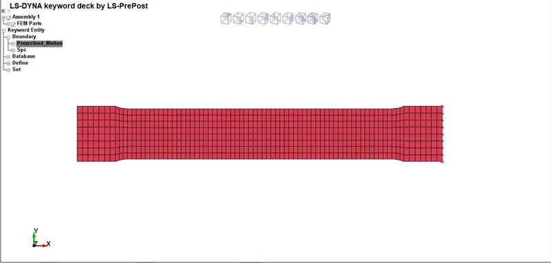
To calculate the displacement for the boundary condition, we know 100 percent strain equals a stretch ratio of value 2.

λ=1+εe">λ=1+εe

εtrue=ln(1+εe)⇒εtrue=ln(2)">εtrue=ln(1+εe)⇒εtrue=ln(2) {Since λ">λ=2}

Strain=(Change in length)/original length

Therefore, Change in length or displacement = ln(2)⋅145=100">ln(2)⋅145=100

λ">λ=Stretch ratio

εe">εe=Engineering strain

εtrue">εtrue=True strain

This value has been assigned to the load curve scale factor also a load curve has been created to define the displacement.

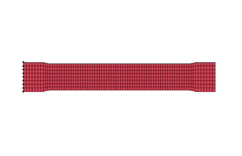
The nodes at the other end of the model are fixed in all DOF except at translation along the y-axis using single point constraint(SPC).

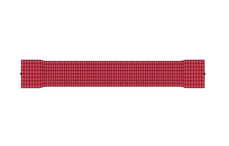
Also, two more nodes are constrained only in the y-direction as shown in the figure below to describe the actual behavior of the model.

5.Defining control cards for implicit analysis.

*CONTROL_IMPLICIT_GENERAL: The keyword makes sure that the analysis will start in an implicit manner since the default analysis mode for ls dyna is explicit. Here the IMFLAG is set to 1 to activate the implicit analysis.

*CONTROL_IMPLICIT_AUTO: Used to change the time step for the given problem. In implicit the time step can be changed since its unconditionally stable but in explicit analysis, the time step is the condition beyond a certain value. Here IAUTO value was kept as one.

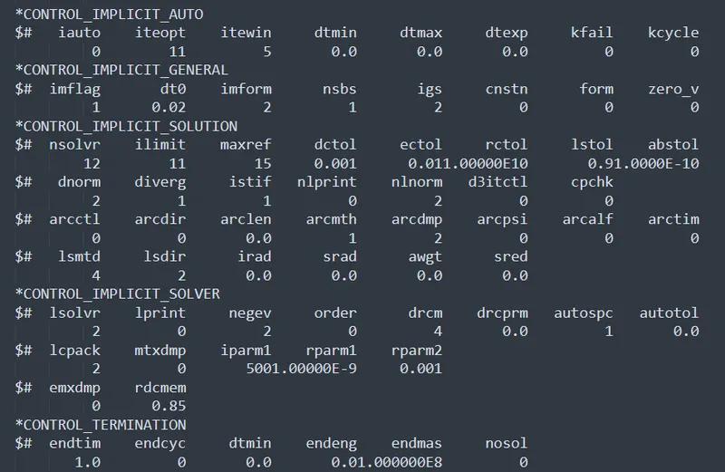
Apart from this other cards such as *DATA_BASE_EXTENT_BINARY, *DATABASE_ASCII, and BINARY_D3PLOT were created to get the required outputs.

The end time was defined as one using the *CONTROL_TERMINATION card.

6.Defining material and section to the part.

Section: Section card is defined for the model.

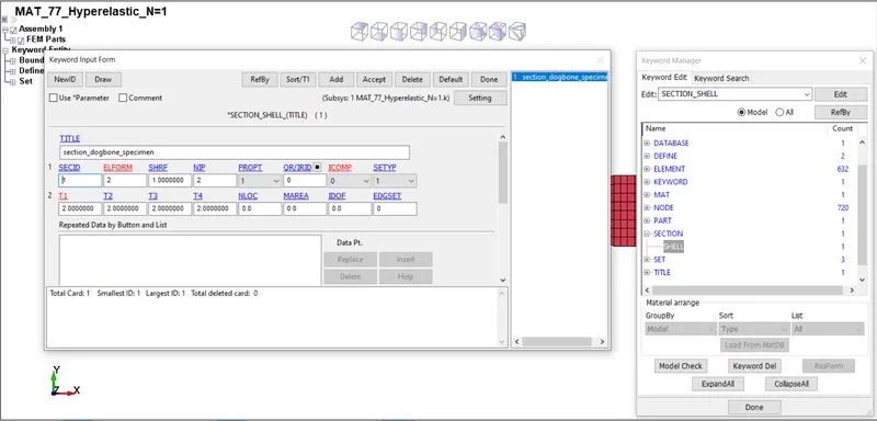
Material:

CASE-1 MOONEY RIVLIN

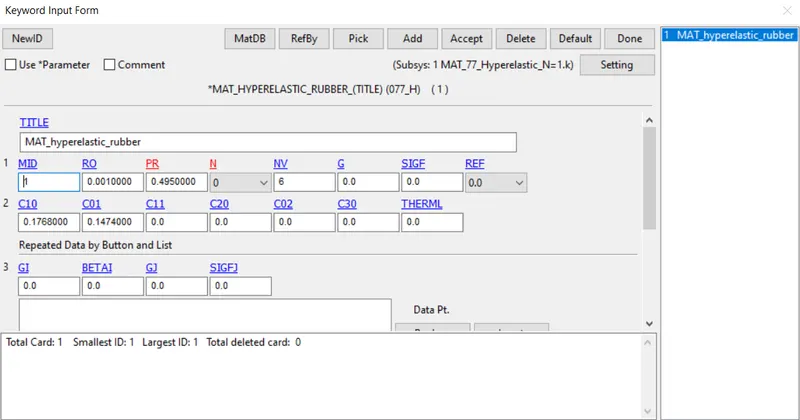
*MAT_HYPERELASTIC_RUBBER(077_H) card was used while modeling the specimen in first case. Other parameters such as density, Poisson's ratio, N (Number of constants to solve for) LCID were also assigned. The LCID was assigned with the data taken from the excel sheet. It can easily be assigned with the help of Text Editor.

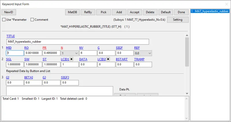
• Initially, the value for N in the material card was kept as one and it been changed to two and three after each run and found out the constants needed for the final run.
• From the Ls-dyna manual, it's said that Load curve ID giving the force versus actual change in the gauge length. If SGL, SW, and ST are set to unity (1.0), then curveLCID1 is also engineering stress versus engineering strain.

after running the simulation, cofficient can be found from the d3hsp.

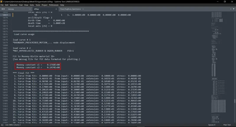
now define the hyperelastic material using the coffiecient which is found using above steps.

N2
c10	c01	c11	c20	c02
0.2595	0.04594	-0.02092	0.002913	0.001016

N3
c10	c01	c11	c20	c02	c30
0.2611	0.0442	-0.006076	-0.002667	-0.009966	1.57E-04

CASE-2 OGDEN

Curve must be defined using DEFINE_CURVE same as explained in mooney rivlin now we only have to define ogden material using MAT_77_O card.

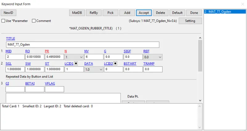
After running the file cofficient can be found using the d3hsp and define the OGDEN material using the cofficient.

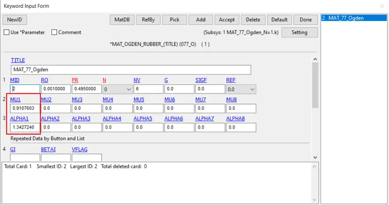
simmiliar way cofficient can be found for N1, N2 , N3.

N1

mu1

0.91

alpha1

1.3427

N2
mu1	mu2
0.9156473	2.225956
alpha1	alpha2
1.339909	0.0018435

N3
mu1	mu2	mu3
-0.0318426	0.2613754	0.6819919
alpha1	alpha2	alpha3
1.926318	1.550334	1.288785

Simulation:

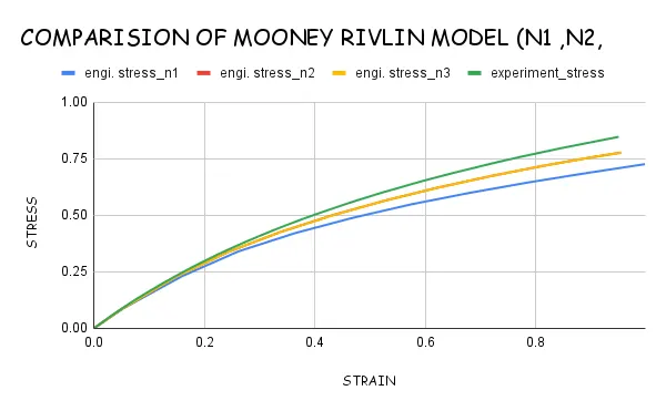
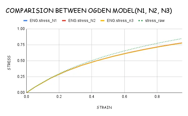
from the above case we get true stress and true strain. we can convert it into engineering stress and engineering strain and compare with the raw data.

CONCLUSION:-

1. The Mooney-Rivlin and Ogden material constants are obtained from d3hsp file by inputting the value of polynomial N=1 in the material card MAT_77_H and MAT_77_O.
2. The stretch stress curve data obtained from d3hsp for both hyperelastic constitutive models were verified with experimental material data and found to be a close fit.
3. The simulation results of tensile test for both material models with experimental data showed a slight deviation due to high non-linear behaviour of the given hyperelastic material and the generic values of density and Poisson’s ratio.
4. From the simulation results, both hyperelastic constitutive material models were found to be valid to describe the behaviour of the given material data.
5. The Ogden material model has more polynomials ranging from 1 to 8 and is easy to use and gives better adjustment to experimental data at the cost of computional time.
6. Learned to verify and validate hyperelastic material model for the given material data.