Week 1- Mixing Tee

OBJECTIVE :

To setup steady state simulations and to compare the efectiveness of the mixing Tee when hot and cold fluids enter at given temperature and velocity. This corresponds to further study of the difference between using K-epsilon and K-omegaa SST variance for the turbulent model.

Cases are given to study for different momentum ratio of cold fluid entering the pipe.

1.SHORT TEE

Turbulence model types :

• RANS (Reynolds average Navier stokes simulation)
• LES (Large Eddy simulation)
• DNS (Direct Numerical simulation)

From this above mentioned turbulence types , RANS is widely used under computer applications and considered more reliable and easy. These RANS can be classified into K-epsilon ans K-omega SST types and each of the types has its own significance.

SIMULATION OF MIXING TEE ( when momentum ratio =2 )

given data

momentum ratio = 2 so cold velocity would be 6 m/s

Temperature at hot inlet - 36 C

Temperature at cold inlet - 19 C

Simulating the problem for the above mentioned inputs.

ANSYS WORKBENCH

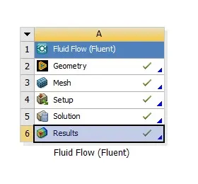
The given problem is solved in ansys workbench using ansys fluent. ANSYS fluent consists of following pictorial presentation as the problem is solved from the geometry to the end CFD post processing.

GEOMETRY

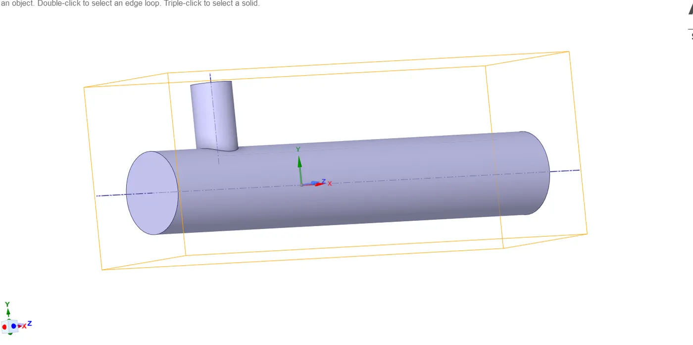
Here the geometry where the simulation takes place is loaded and defined for volume extraction model as the fluid working here interacts only with the inner space inside the volume.

MESH

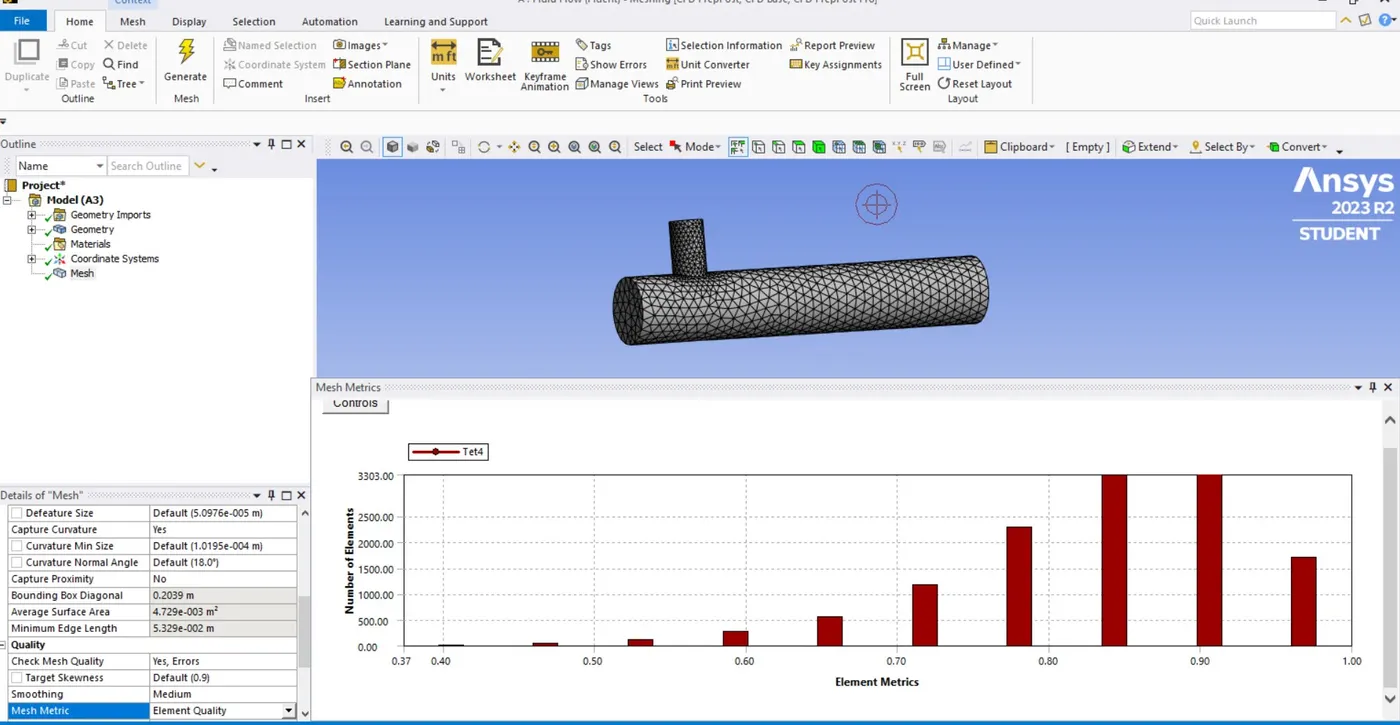
Here the meshing is done and the faces corresponding to hot velocity inlet and cold velocity inlets are mentioned.

SETUP

Here the solving part for the mixing Tee is performed with the acquired physical data and the quantities that are like to be interpreted on the simullation flow. \

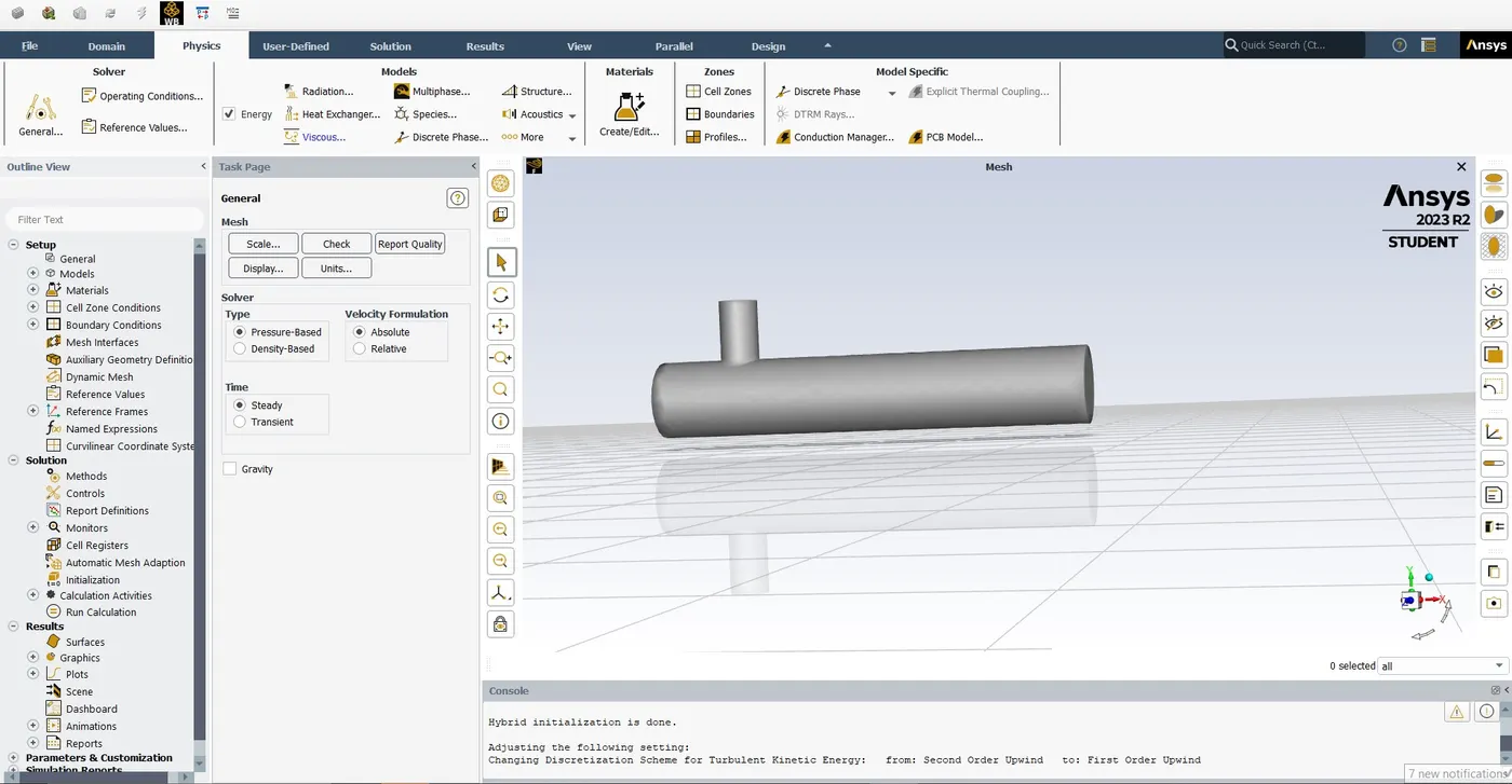
K-epsilon mode of RANS based turbulence mode is used here.

Results after simulation.

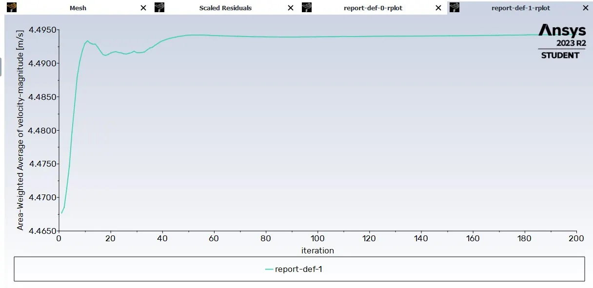
Average velocity line plot

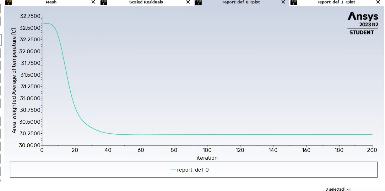
Average Temperature line plot

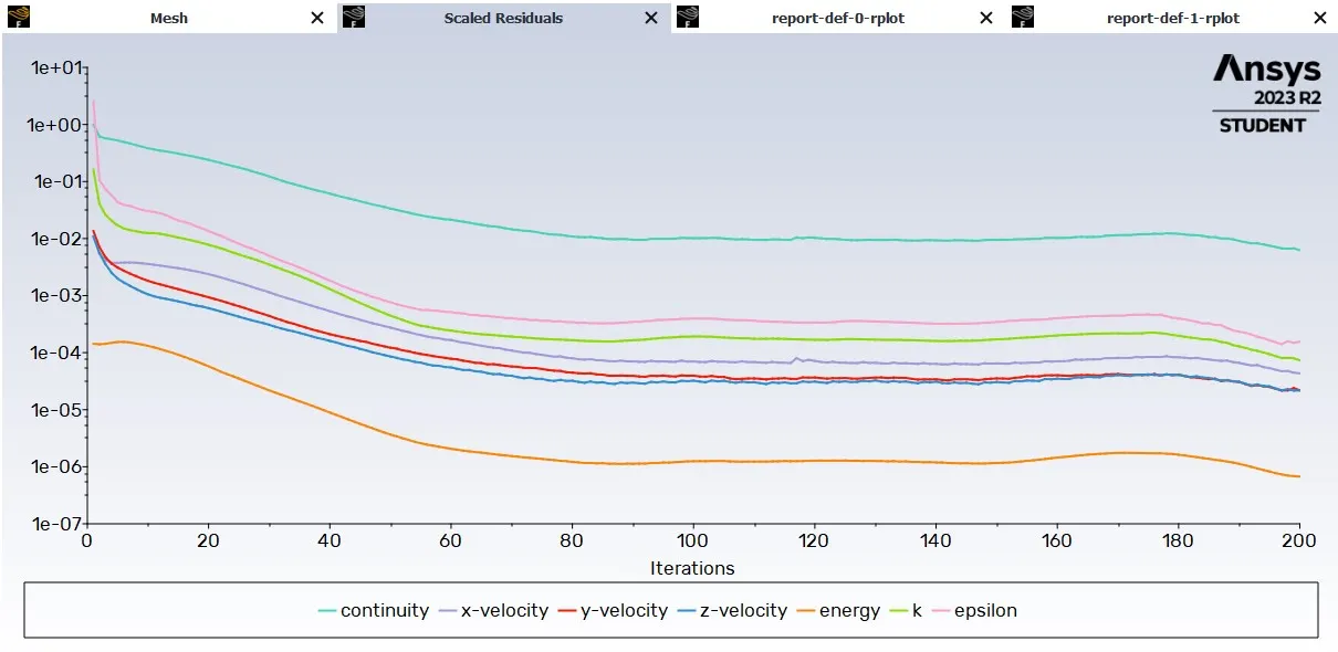
Scaled residuals

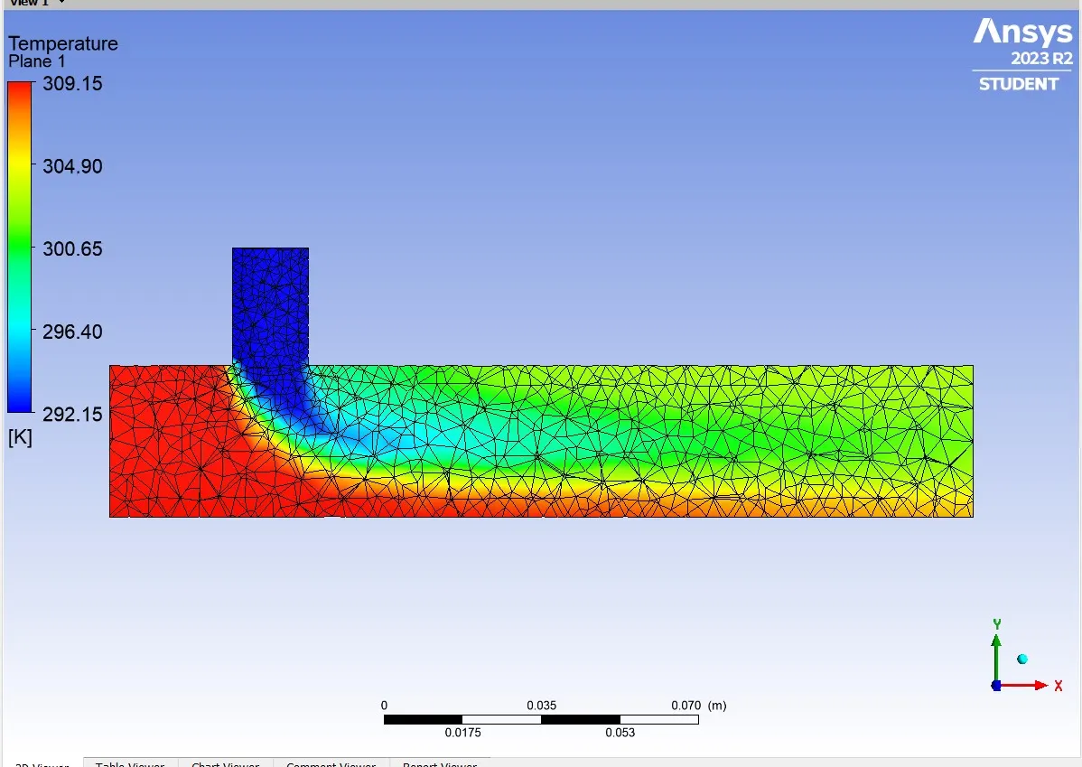
Contour plots - Average temperature

Contour plots - Average velocity

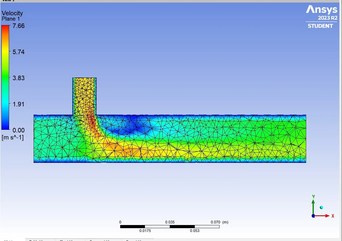
Solving the same geometrical meshed mixing Tee for K-omega SST mode of turbulence.

Here the setup goes a bit different as the turbulence mode specified is K-omega SST. Changing the turbulence mode and maintaining other inputs as unchanged the simulation performed gives results as below.

Average temperature line plot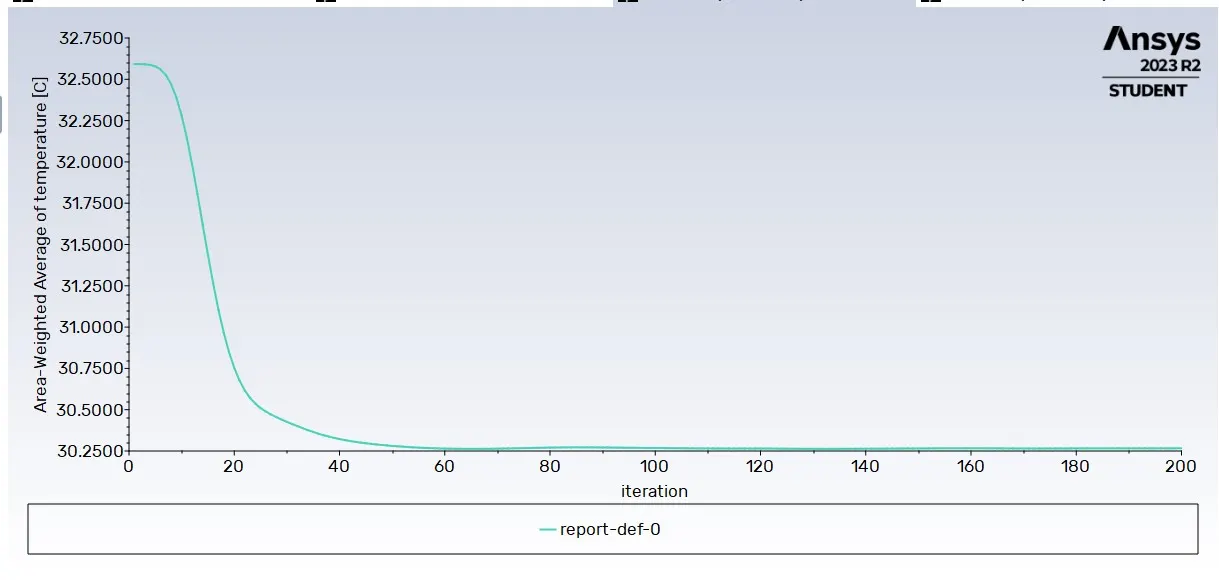

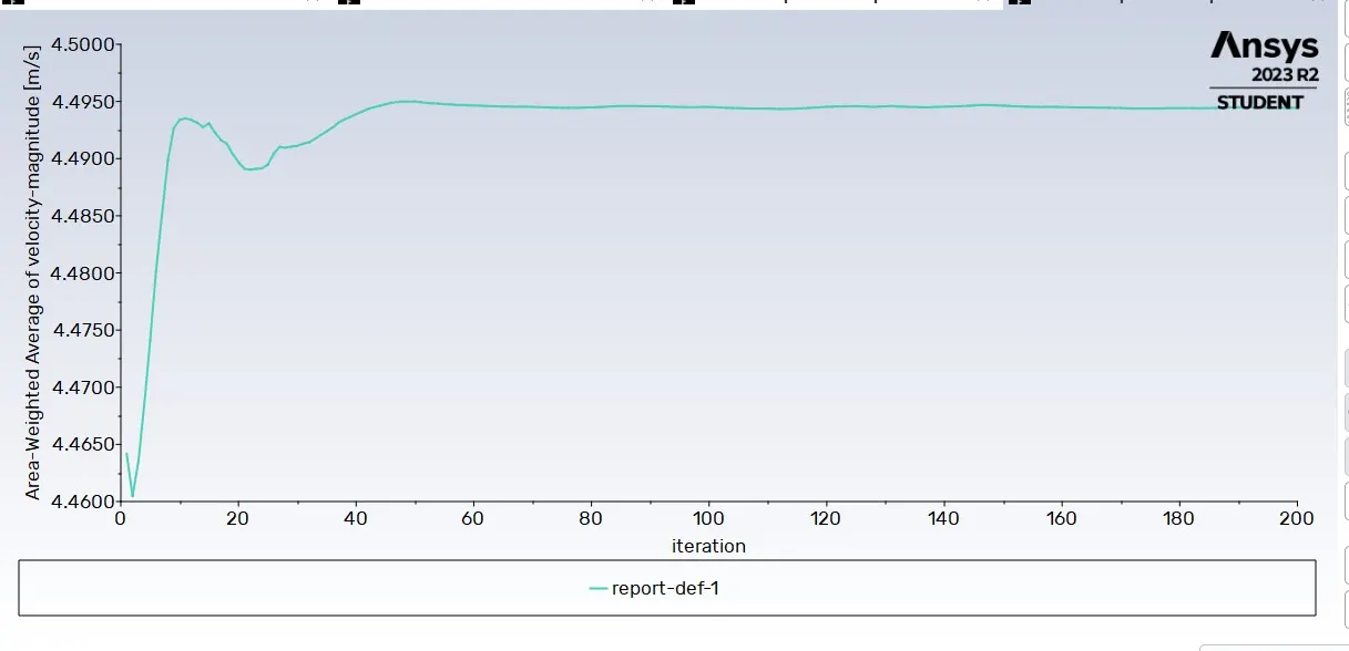
Average velocity line plot

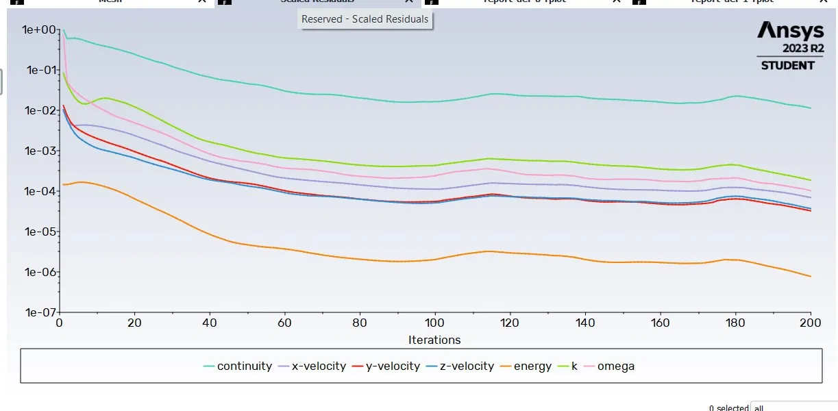
Scaled residuals

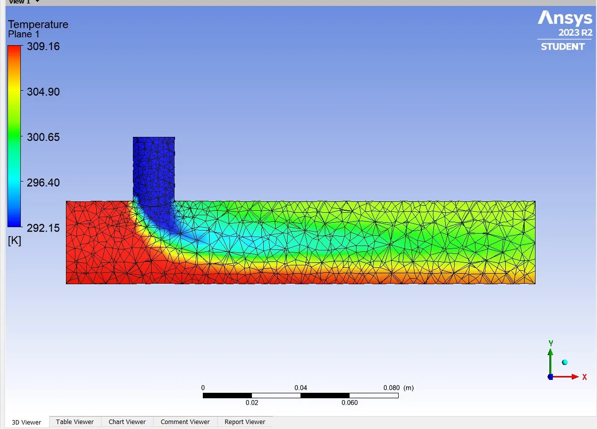
Contour plots - Temperature

Contour plot - Velocity

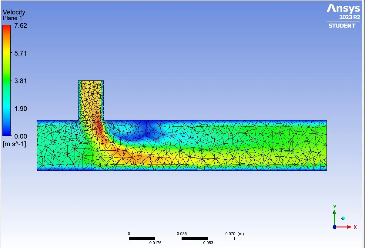
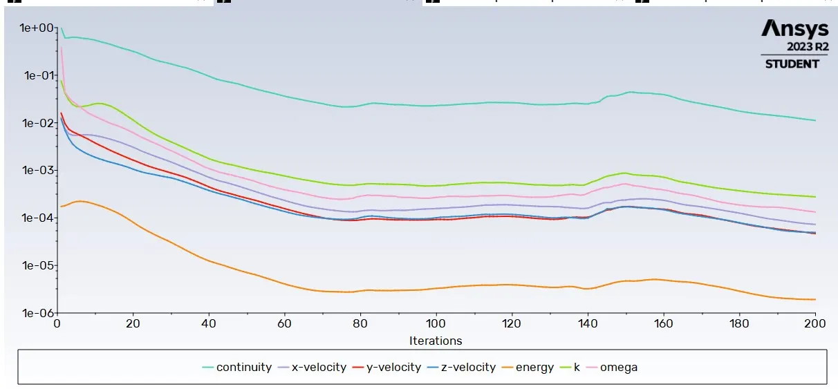
By comparing the results of scaled residuals K-omega SST gives a smooth transistion in approximating the values as the graph of the residuals show a linear phase whereas in K-epsilon the graph is wavery for approximating the values. For further simulation of Long Mixing tee K-omega SST mode of turbulence variance is used.

SHORT TEE ( momentum ratio = 4)

Changing the momentum ratio i.e the cold velocity value to 12m/s in setup option in ANSYS FLUENT results in different silmulation study of the mixing Tee. As one of the influencing parameter of solving physical data has been changed.

This solution falls into the results of

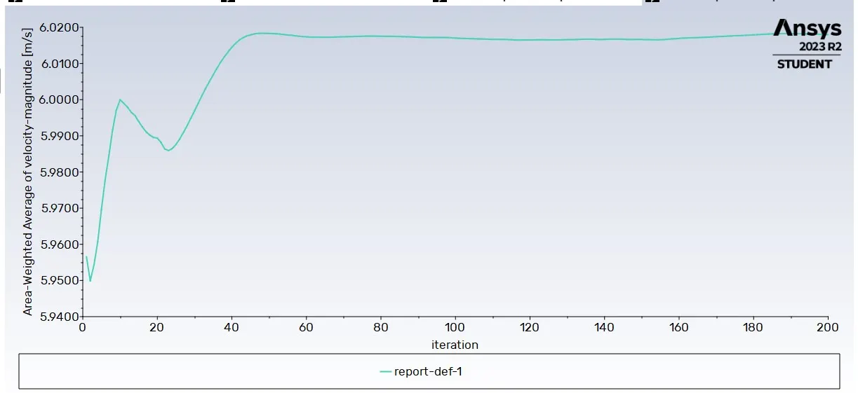
Average velocity at the outlet

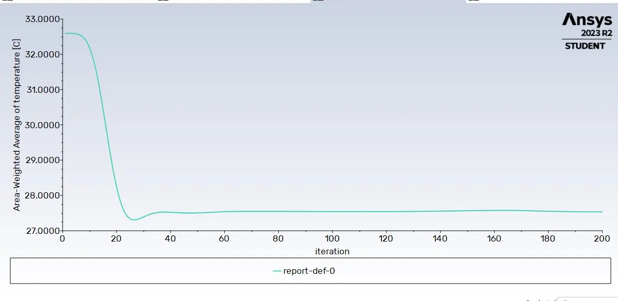
Average temperature at outlet

Scaled residuals

Contour plot - temperature

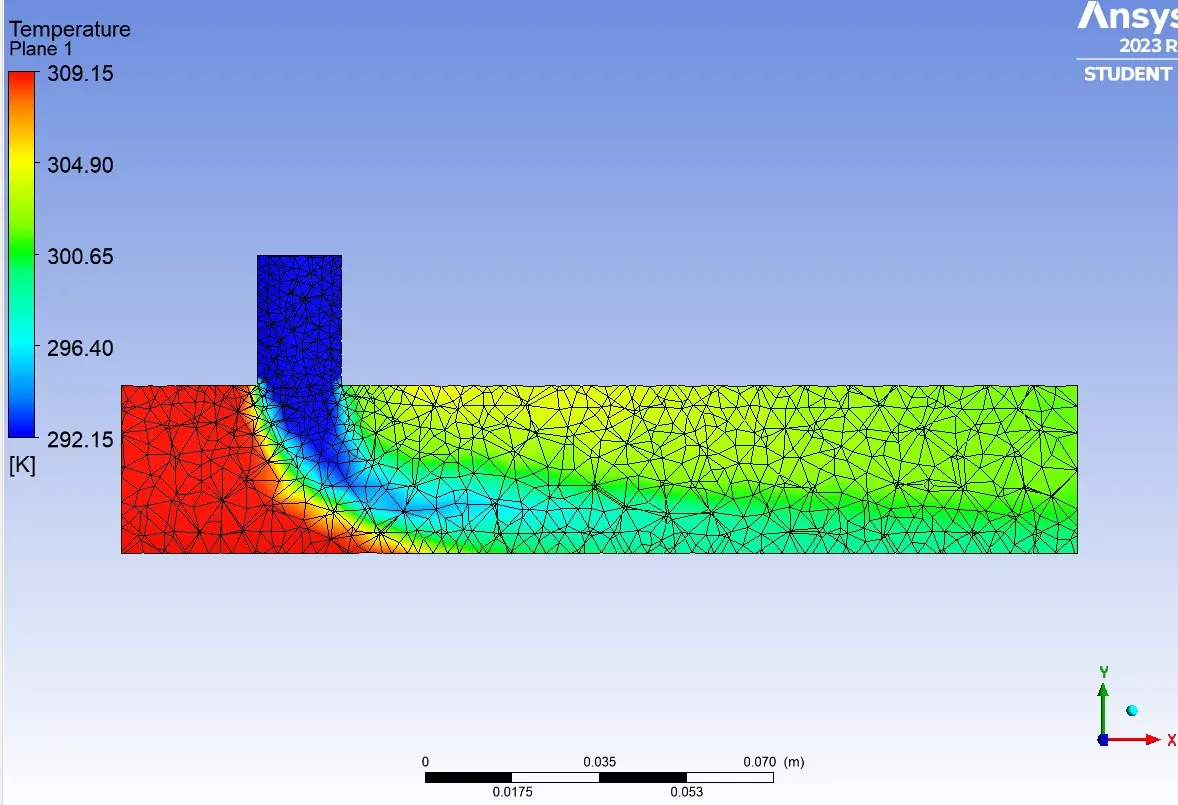
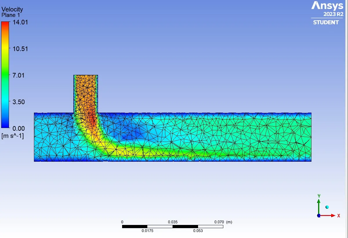
Inference: Here the cold fluid entering at a larger velocity (12m/s) when compared to older one (6m/s) creates a major impact in the simulation as in the contour plot it is clearly visible, the cold air impacts much stronger resisting the hot air a way more and influencing to produce much lower average temperature at the outlet around 27.5 C. This impacts not only for resulting temperature but also for the velocity. As the velocity at the outlet is increased to 6 m/s , Initially it was around 4.49 m/s for the setup ( momentum ratio = 2).

Contour plot - velocity

LONG TEE

Here the geometry of the mixing Tee is changed and so does the mesh, setup and the end results. Same solving criteria , the physical data inputs and the definitions for the turbulence is set to K-omega SST variance. This gives the end results as follows

GEOMETRY

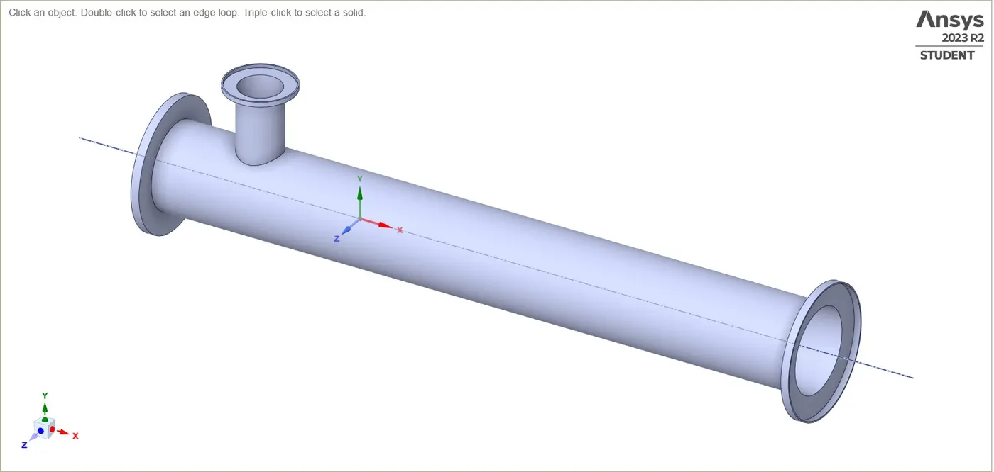
LONG TEE with mesh quality elements

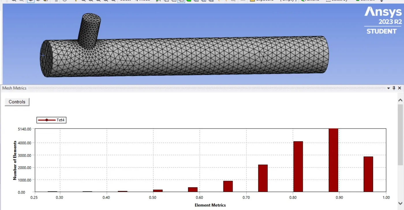
LONG TEE solved when momentum ratio is 2

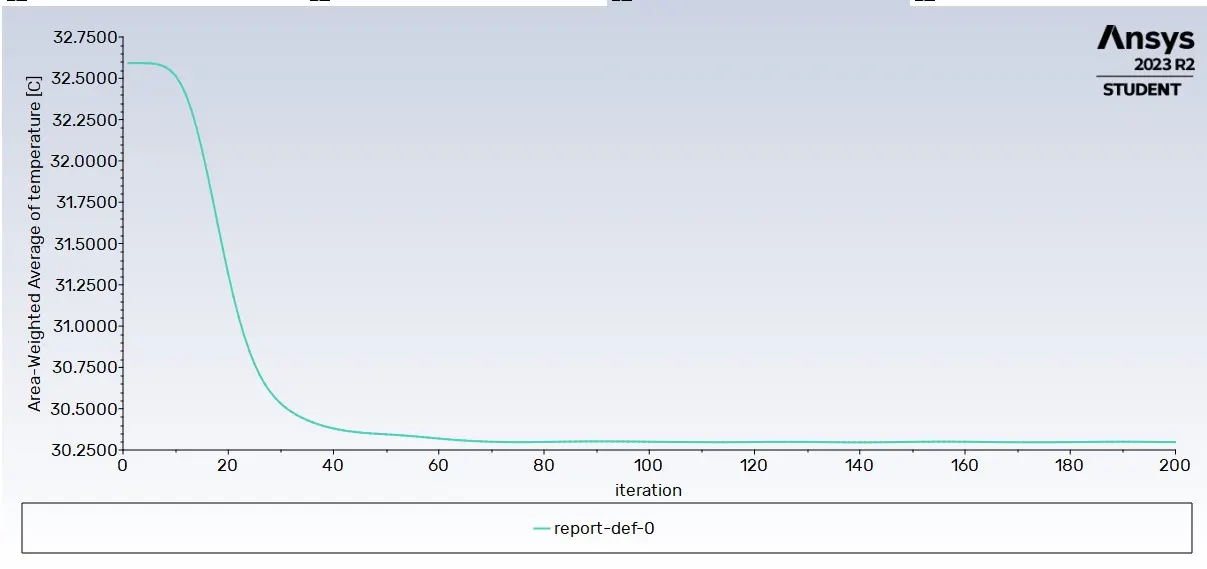
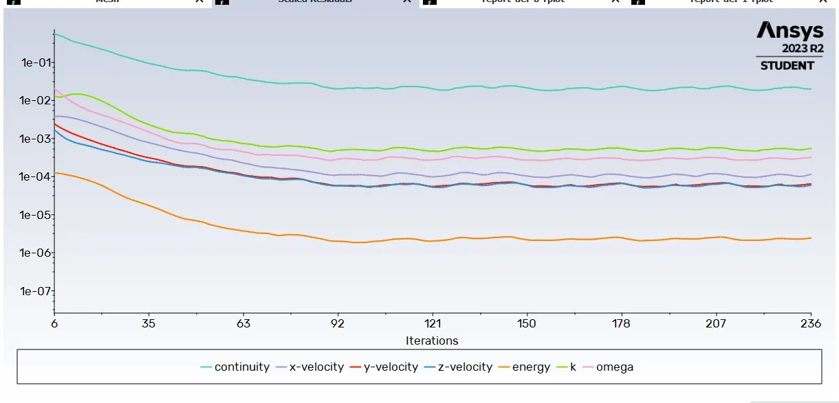
momentum ratio = 2, therefore the inlet velocity at the cold part would be 12m/s. Involving this cold velocity and solving for the geometry for Turbulence K-omega SST mode , results interpreted as follows.

Average velocity at the outlet -line plot

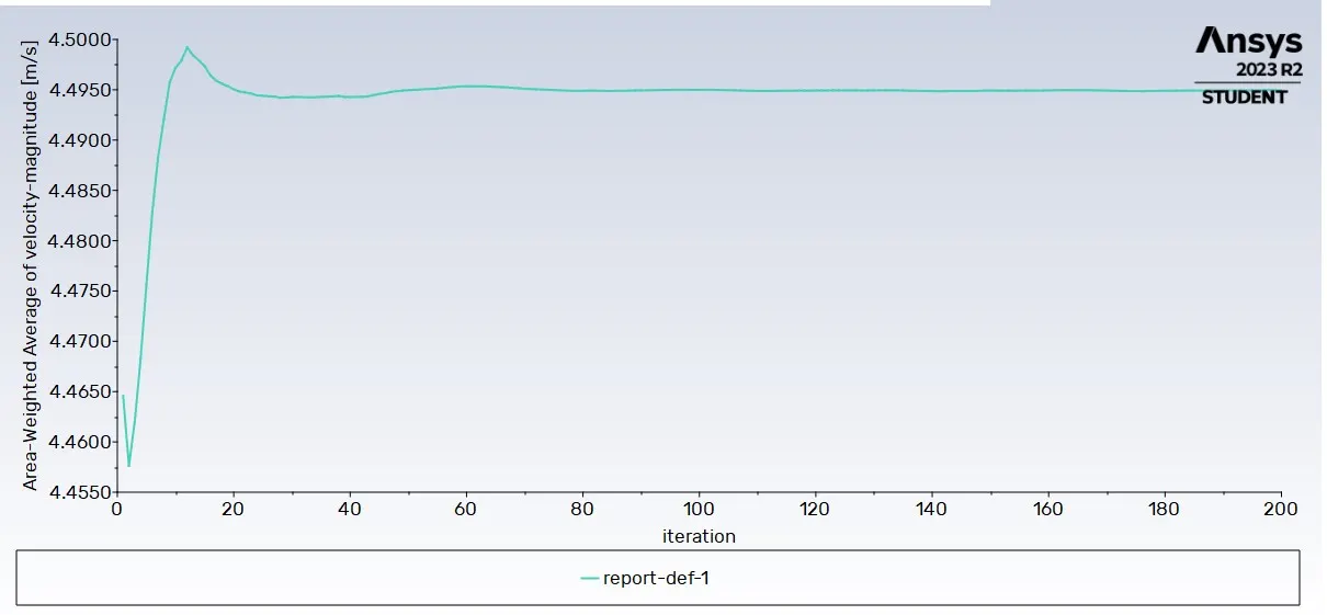
Average temperature at the outlet - line plot

Scaled residual

Contour plots

Average temperature at the outlet

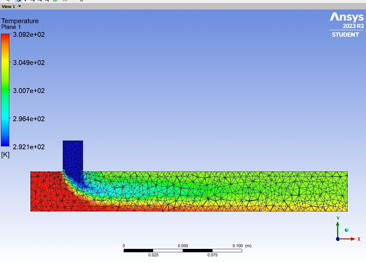
The hot air gets influenced and bounded towards the boundry as the cold inlet air pushes it away

Average velocity at the outlet

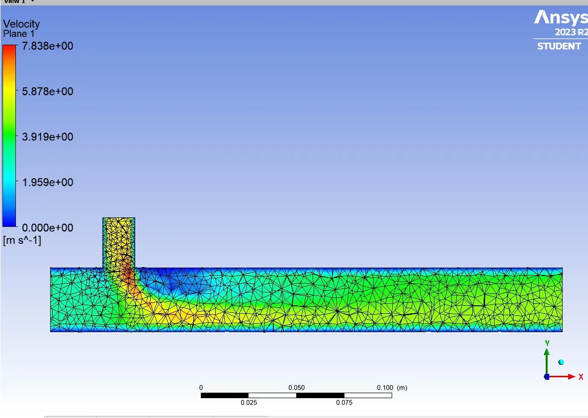
LONG TEE (momentum ratio = 4)

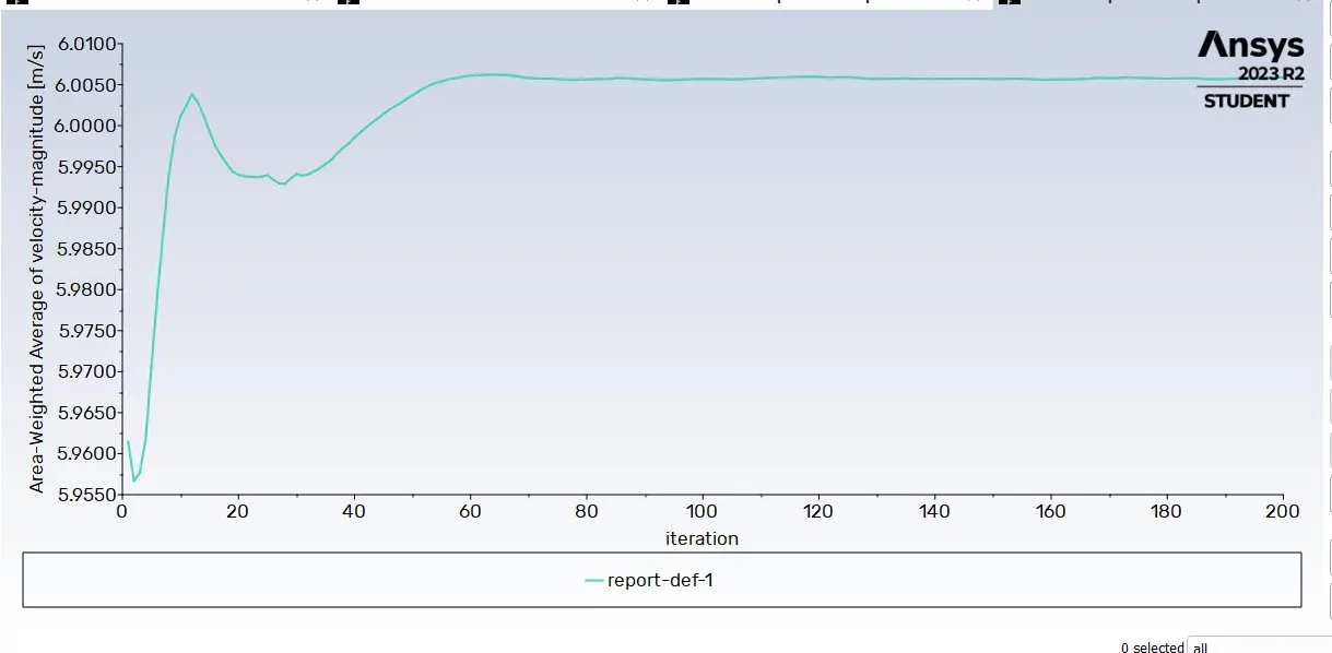
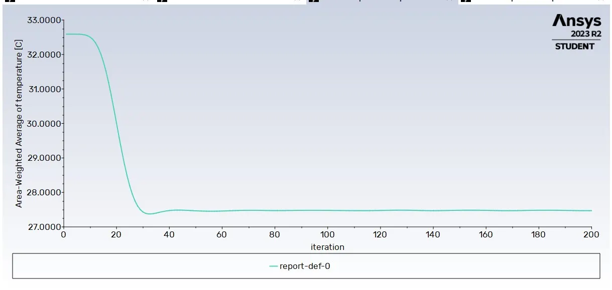
By changing the cold inlet velocity , the simulated end resuults for the geometry goes significantly varied as the inlet cold velocity influences the temperature change and average velocity cahnge at the outlet.

GRAPHS and PLOTS

Average velocity at the outlet

Average temperature at the outlet

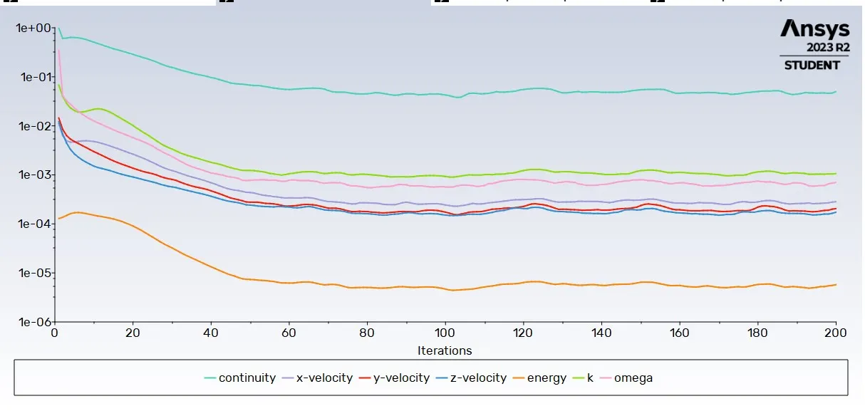
Scaled residuals

Contour plots

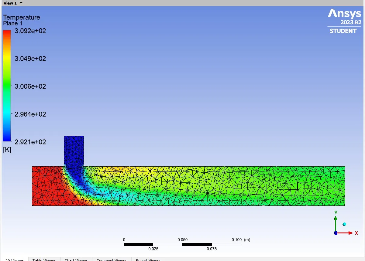
Average temperature

Average velocity

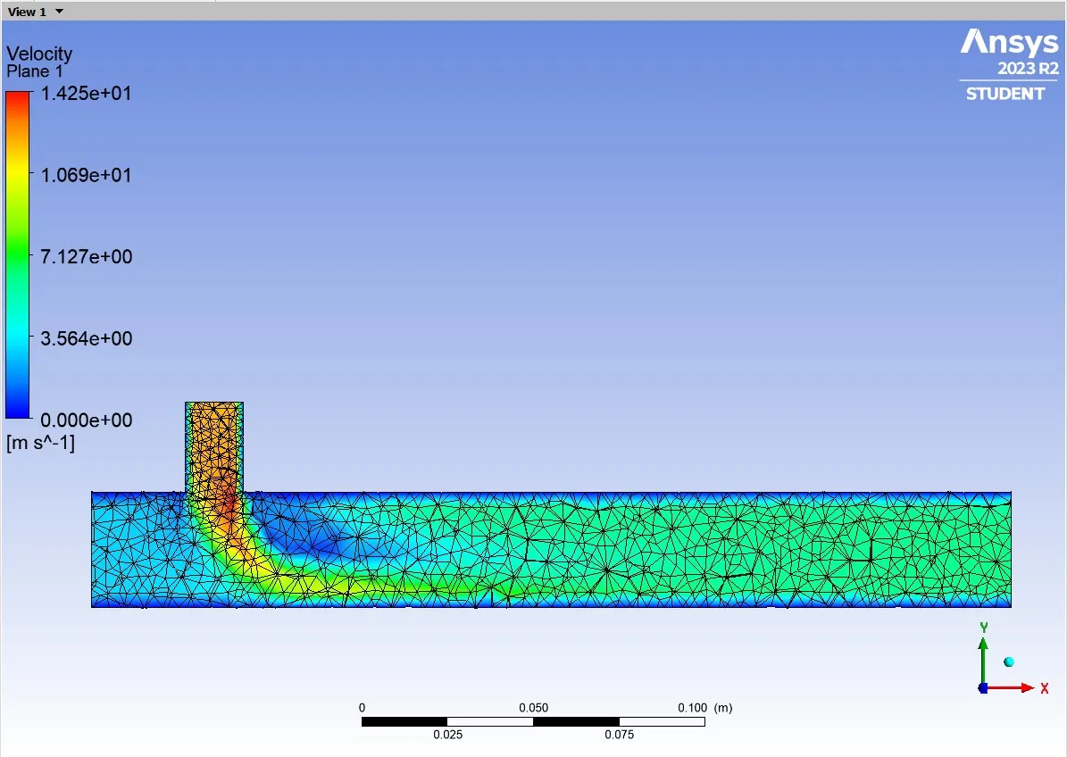
Inference : The fluid coming out from the Long Tee(momentum ratio = 4) has lower average temperature and higher velocity, This is due to the impact of the cold air entering at a velocity of 12m/s influences the hot air to gain some speed and decrease its temperature.

Considering the momentum ratio as 4 comparison of Short Tee and Long Tee is done

	SHORT TEE	LONG TEE
CELL COUNT	12613 cells	15561 cells
AVERAGE TEMPERATURE AT OUTLET	27.5 C	27.5 C
NUMBER OF ITERATIONS FOR CONVERGENCE	70	80

CONCLUSION :

• Cold air velocity influences the hot air flowing inside the pipe and the velocity variance impacts the average temperature and velocity at the outlet
• As the mesh size is refined the number of iterations and time taken to converge is increased as the governing equations has to pass and solve for every cells present inside the Mixing Tee pipe .