Week 1- Mixing Tee

Aim:Mixing tee on short and long mixing tee of hot inlet velocity 3m/s.

Introduction:

The mixing tee, is commonly employed where two fluid streans with different physical propeties mix together, for example petroleum indusry, HVAC systems.The effictiveness of mixing Tee can be defined in terms of unifromity of properties at the outlet, for example temperature,velocity.The fluid propeties at both the inlet have different temperatues and velocities difference lead to heat transfer and the final mixture attains a steady unifrom temperature.

The leangth of the pipe is also a factor to consider. Pipe length affect the development of flow pattern. the flow usally becomes turblent in longer pipes which helps in effective mixing of fluid.

Theory:

Computationa Fluid dynamics is a branch of fluid dynamics,which is used to mathematical physics and computationa software to undestand how the flid flow effect in desired surface to visualize.CFd mostly used to predict the fluid flow phenomena using governing equations like Navier stokes equations.in this study we are going to using the ansys fluent software.In the ansys workbench we have to perform all three major steps in simulation pre-processing,solving,post-processing.Ansys fluent used for incompressible flow,compressible flow,turbulence,Multiphase,heat transfer. 

Mixing tee is a device which uses specifically engineering internal geomentry to mix two fluid strames into one steam, efficiently.In this sudy we have take hot and cold air to take different temperature, velocities.We will use two different mixing tee distinguished with length and analyse the effect of mixing tee.

Solving & Modal Approch:

We take the Two 90 degree mixing tee of different length are considered to evaluate the effect of geomentry on the effectiveness of mixing steady-state simulations conducted to compared mixing tee effectiveness.take the hot inlet temeperature is 36 deg &the cold inlet is at 19 deg.Also, the effect of inlet fluid velocities on the mixing effectiveness is compared for different cold-hot fluid inlet velocites ratio's.

Case1:

Short mixing tee with a hot  inlet velocity of 3m/s.

momentum ratio of 2,4

Case2

Long mixing tee with a hot  inlet velocity of 3m/s.

Momentum ratio of 2,4

momentum ratio=Velocity at cold inlet/velocity at hot inlet.

Numerical solution in outlet

Where m=density*area*Velocity

density=1.225 kg/m^3

Area of cold inlet=0.0002m^2

Area of hot inlet=o.ooo9m^2

From momentum ratio 2

T mixture=30.76deg C

From momentum ratio 4

T mixture=27.78deg C

Pre-Processing:

• Let start with the analyzing the best method to converge the solutions, understand the k-epsilon andk-omega SST modal for the mixing tee.

Gomentry:

• Intially open the workbench and using analysis system to open the ansys fluent.

               

•    After click the ansys fluent open gomentry and import the mixing tee.To right click and open the spaceclim.

             

                                 

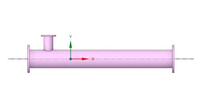
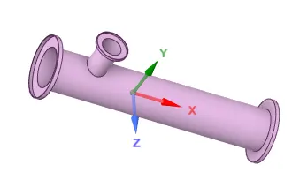
•     We are to analyse the mixing of two fluid, so there is role of parts other than two pipes. to supress that we need to extract volume tee. Go to prepare menu and click on volume exract.Switch to edge selection and select the three outer edges and crate a  volume.

                                   

                                   

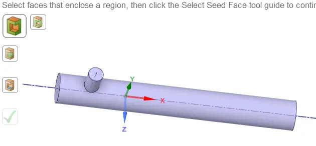
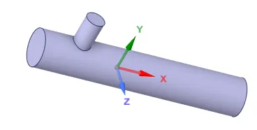
• After create the volume to observe the structure and hide the solid body to uncheck andE suppress for physics.

            

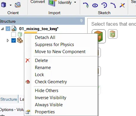
• Exit the spaceclim and clickon mesh to open mesh.

                           

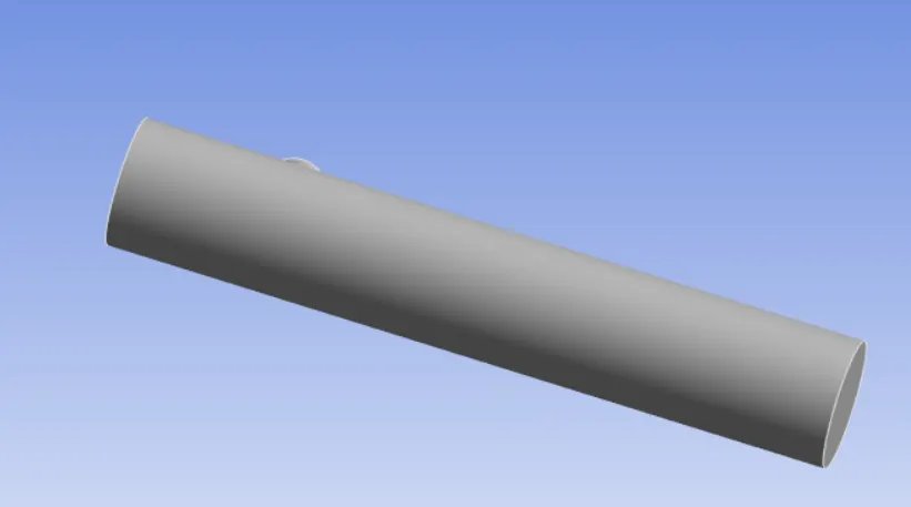
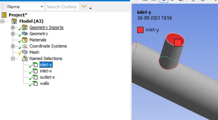
• Open the mesh using the face option to select the each face and create names in all faces.

                         

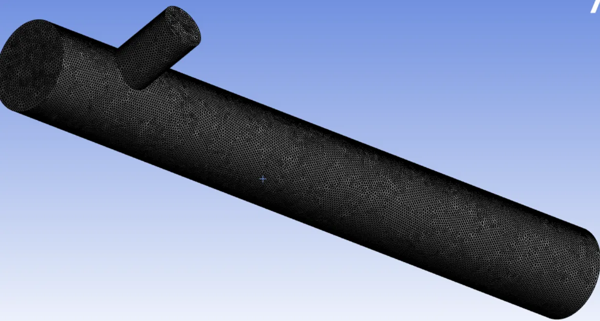
• Now click the mesh option and down to see deatils of mesh.in this we see the sizing, quality etc.Right click the mesh and click on mesh generation it is automatically create the predefined mesh.Change the mesh perameter to see the element size can select and giving the require mesh perameter and right click the mesh to generate the mesh.

                        

• Select the quality ro mesh metric option to select the element quality.

                       

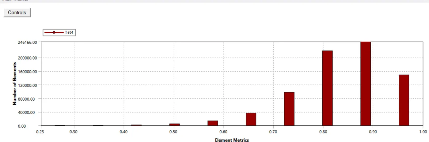
• Exit to the mesh and update the mesh Open the setup.

                            

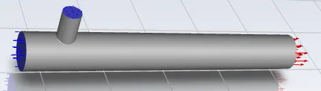
• Intially to check the mesh, in the console we can observe mesh error.

                        

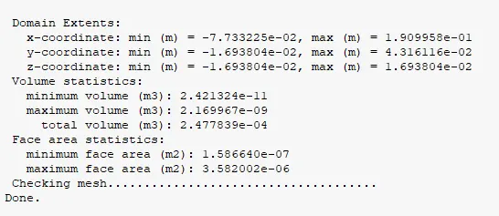
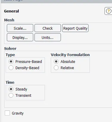
• To open the physics and go to the general mesh solver-pressure base,Velocity Formulation-Absolute,Time-steady.

                          

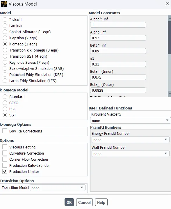
•  Intially to enable the energy.After open the viscous modal open and click k-epsilon modal and change to realizable and remaing perameters consant.

           

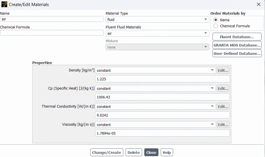
• After going to the materials open the fluent Database to chnge the fluent.In this we not change the fluent our midium is air.

                    

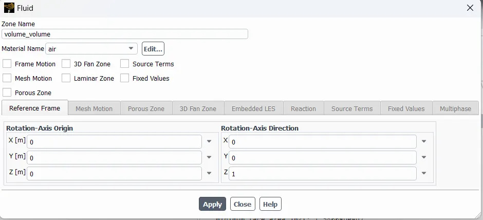
• Cell zone to change the fluent and materials to used.

                      

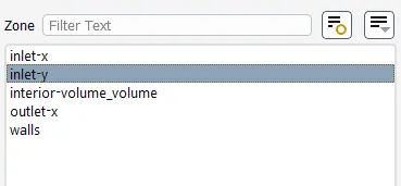
• Now go to the boundaries option to select the inletx giving the temperature 36 deg and velocity 3m/s.Select the inlet y  and assign the temperature 19deg and velocity 6m/s.

               

       

             

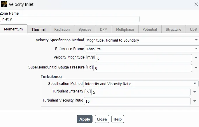
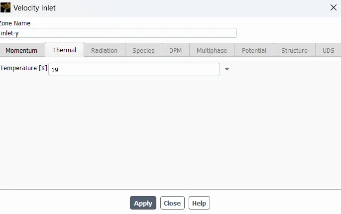
• Open the Sloutions definition option to create new surface reportopen and click the area -weighted average.

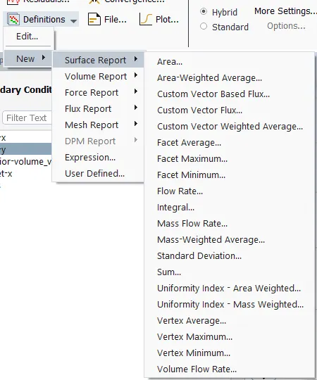
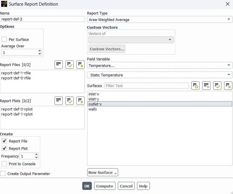
• Area-Weighted average to chnge the feild of varible to temperaraure at outlet and report plot and report file created.

 

• To click the hybrid intilization activate and run the intilization.

           

                                  

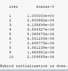
• Run calculation to assign the iteration and cilck the calculate.

• After completing the calculation view the area-weight average and standered deviation and exit the set up.

Post-processing:

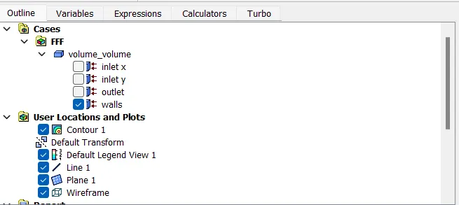
• Open the result and view the left side outline in this we can check the volume and check the wall box.

                   

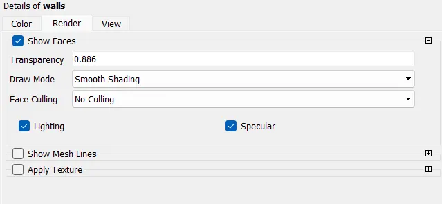
• In the deatiall to change the colar and rendor to transporancy set apply to click.

           

• Plane option to crate the plan in the middle of the wall and click the apply button.
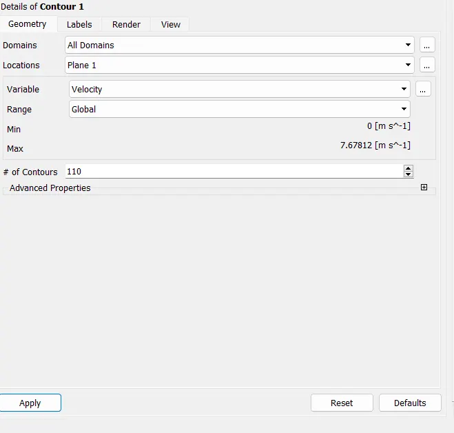
• contour option enable and give the location is plan and varible to change the temperature contours to given and apply.

       

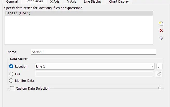
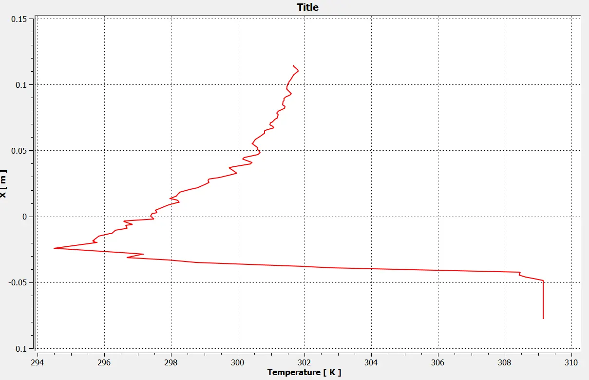
• Location to enable the line and crate the line in x direction in the wall section and apply.
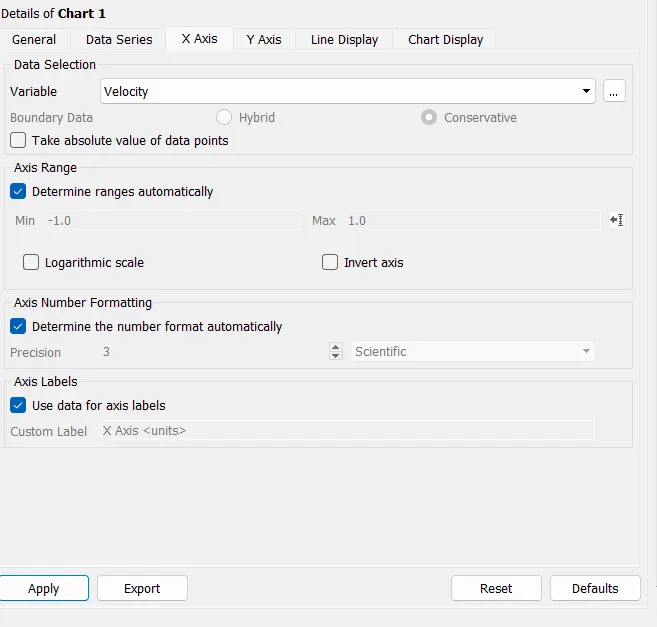
• to view the velocity and temperature line plots enable the graph and giving the location to set the line and chnge the varible in the detais of grap apply view the temperatur and velocity line plots.

         

     

Results:

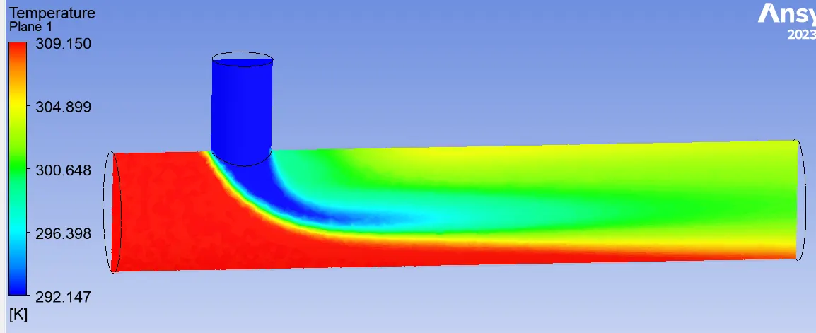
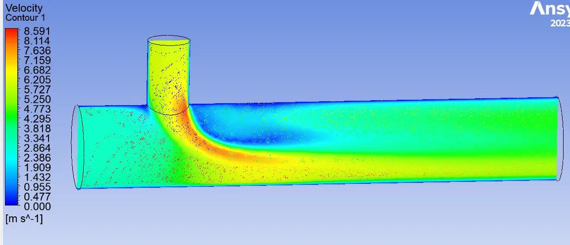
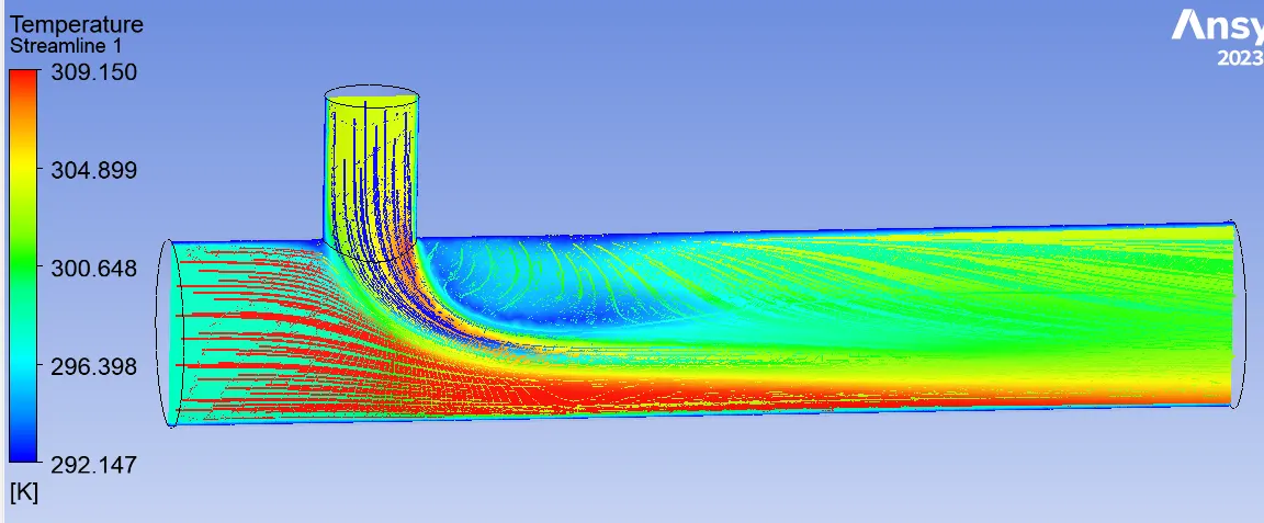
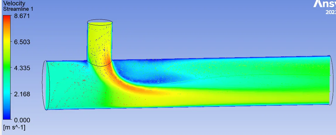
Case1:A

Short Mixing Tee:

Inlet velocity-3m/s

Momentum ratio-2

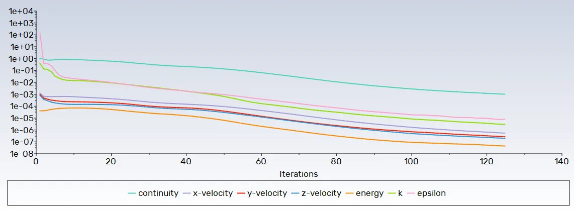
Converge Plot:

The solution is converge into 125 iteration.

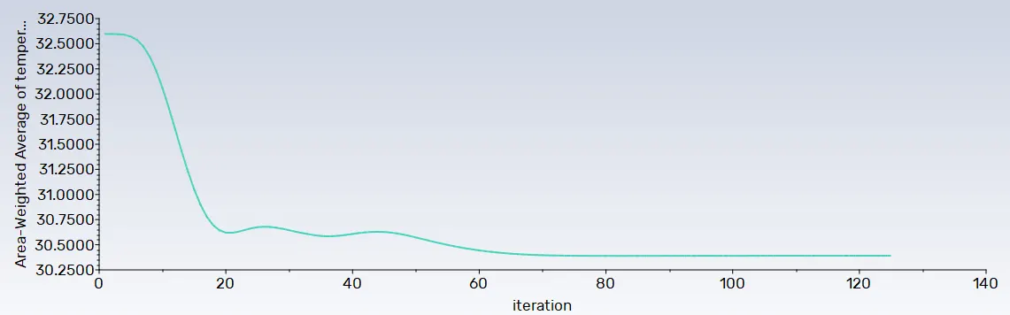
 Area-Weight Average of temperature

The average temperature at outlet is 30.39080C

Temperature contour:

Velocity Contours:

Temperature Steamline:

VelocityStramline:

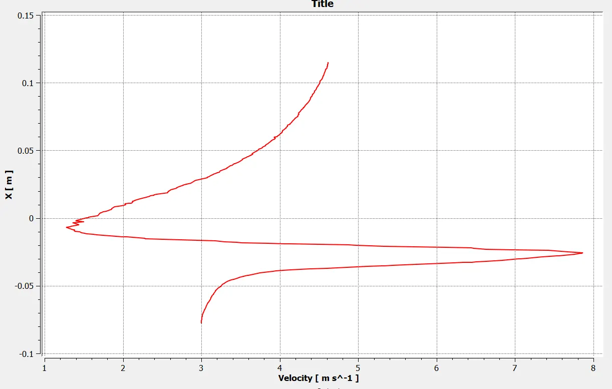
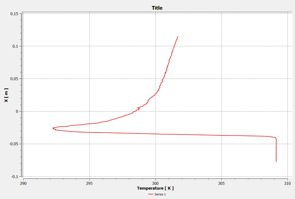
Velocity and temperature line plots

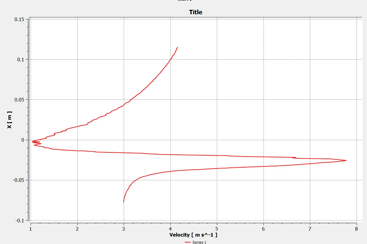
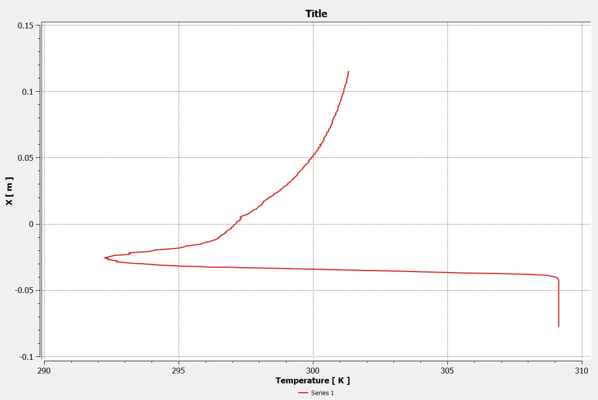
Case1:k-dissipation ratio

Short Mixing Tee:

Inlet velocity-3m/s

Momentum ratio-2

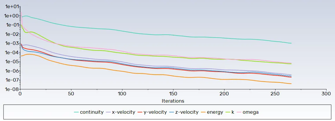
Converge Plot:

The solution is converge into 266 iteration.

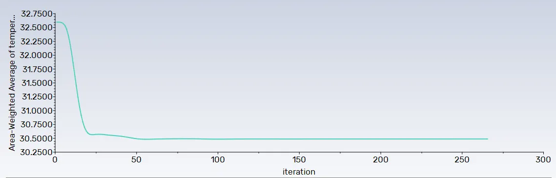
 Area-Weight Average of temperature

The average temperature at outlet is 30.4867C

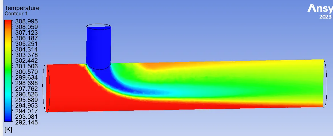
Temperature contour:

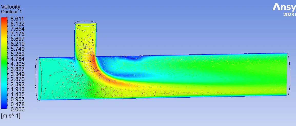
Velocity contours:

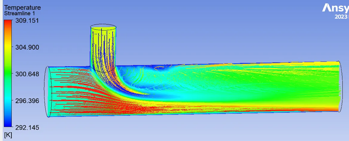
Temperature Stramline:

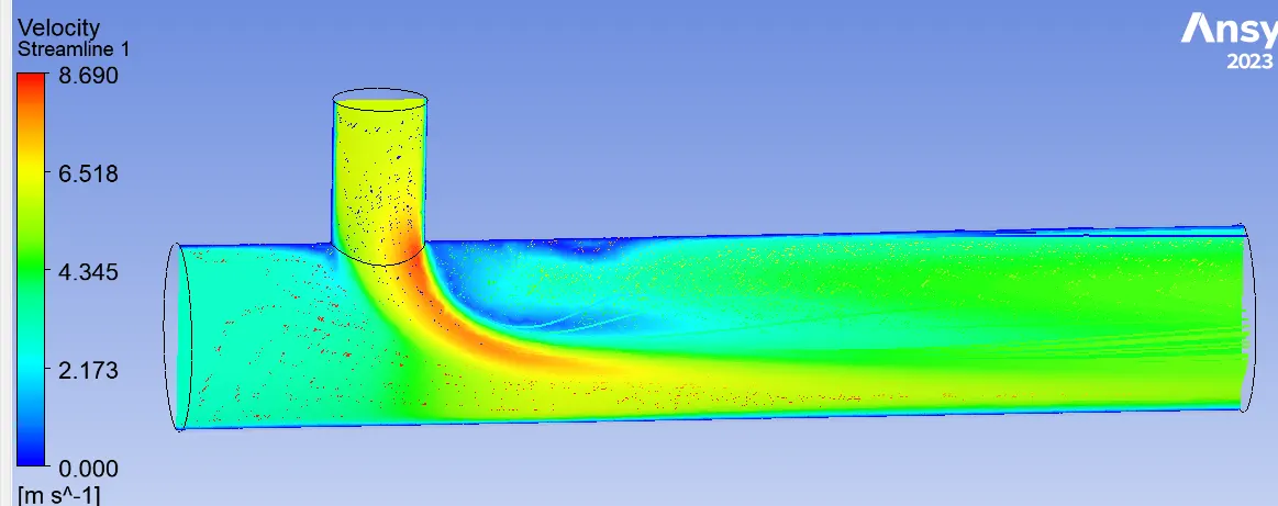
Velocity Streamline:

Velocity and temperature line plot

case                                      k-epsilon                                         k-omega SST

Element                                576190                                          576190

Nodes                                   110523                                         110523

area-weight average              30.39080                                       30.4867

temperature                          309.150k                                       308.995

converge                                 125                                                266

The above table compares the residual convergence and outlet temperature variation for both k-epsillon aand k-omega sst modals.The convergence is said to be attained if the residual value decreases below a certain predefined criteria value and becomes constant in successive iteration or the patteren repeted after sucessive iteration.From the above plots it can be seen that in both the models have convergance criteria.In this case k-epsillon the converge the value at 125 iterations.But in the case of k-omega sst the convergence value 266 iterations.

K-epsilon modal predicts well far from boundaries (wall) and k-omega modal predicts well near the wall.Therfore, the k-epsilon  modal is majority used for free flow away from the wall and as in theis project ,there is no dealing with the wall of mixing tee for change in temperature along the length of it,so k-epsilon modal was for furthre simulations.

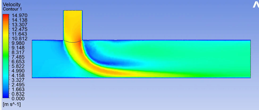
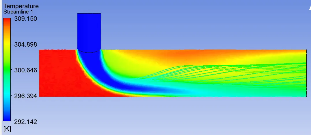
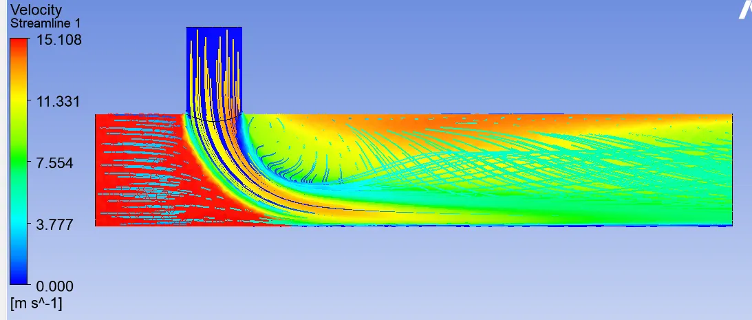
Case1:B

Short Mixing Tee:

Inlet velocity-3m/s

Momentum ratio-4

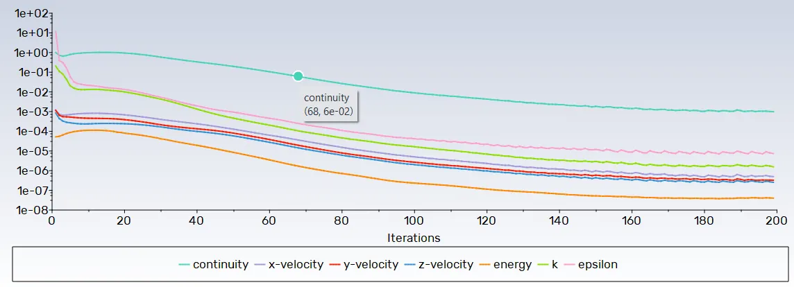
Converge Plot:

The solution is converge into 198 iteration.

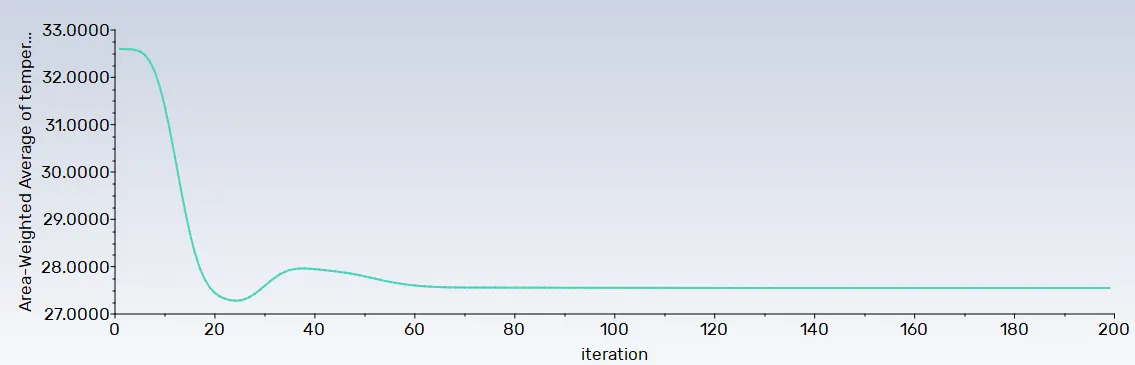
 Area-Weight Average of temperature

The average temperature at outlet is 27.54950C

Temperature Contour: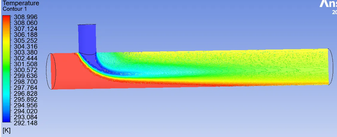

Velocity Contours

Temperature Streamline

Velocity Streamline

Case2:A

Long Mixing Tee:

Inlet velocity-3m/s

Momentum ratio-2

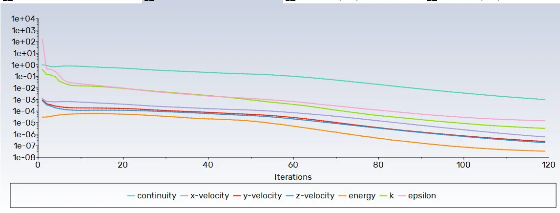
Converge Plot:

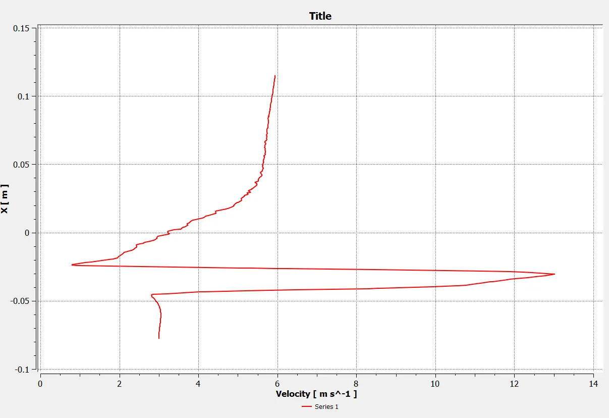
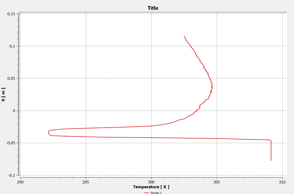
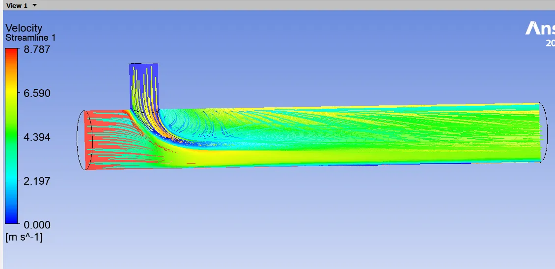
The solution is converge into 119 iteration.

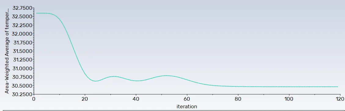
 Area-Weight Average of temperature

The average temperature at outlet is 30.46780C

 

Temperature contors

Velocity Contors

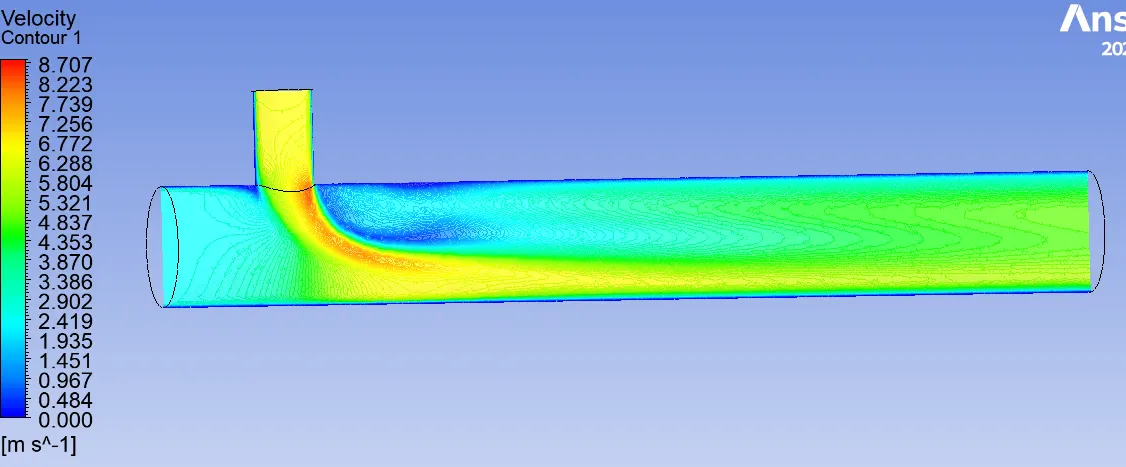
Temperature streamline

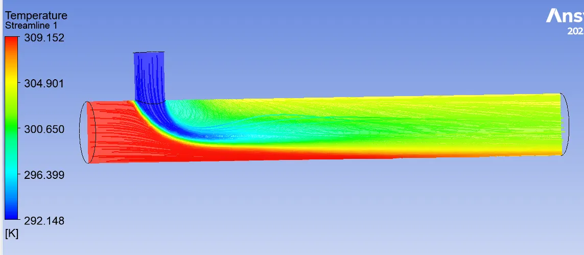
Velocity Streamline

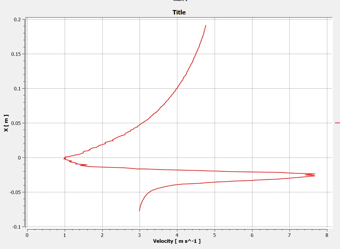
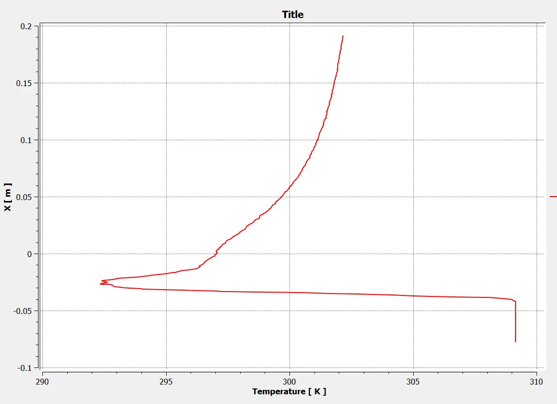
Velocity and temperature line plots

Case:B

Long Mixing Tee:

Inlet velocity-3m/s

Momentum ratio-4

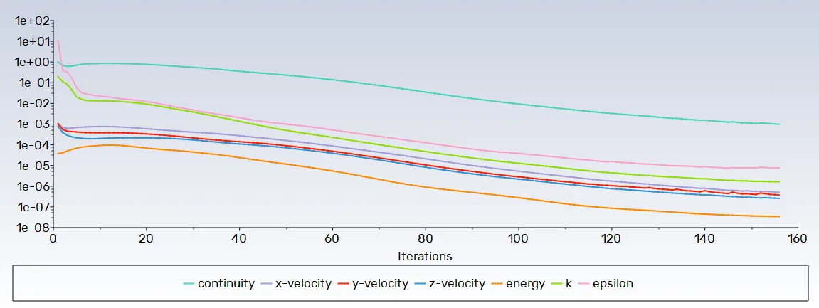
Converge Plot:

The solution is converge into 156 iteration.

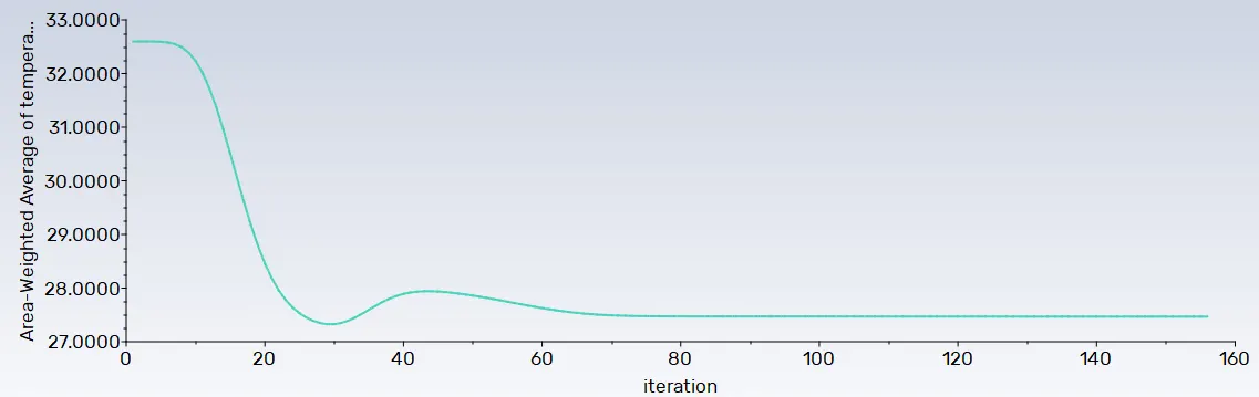
 Area-Weight Average of temperature

The average temperature at outlet is 27.28760C

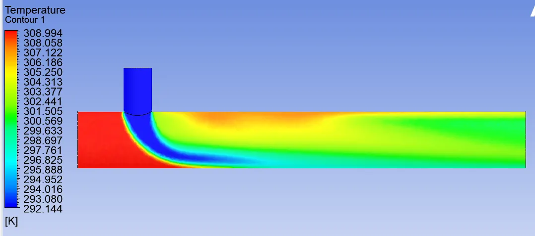
Temperature Contors

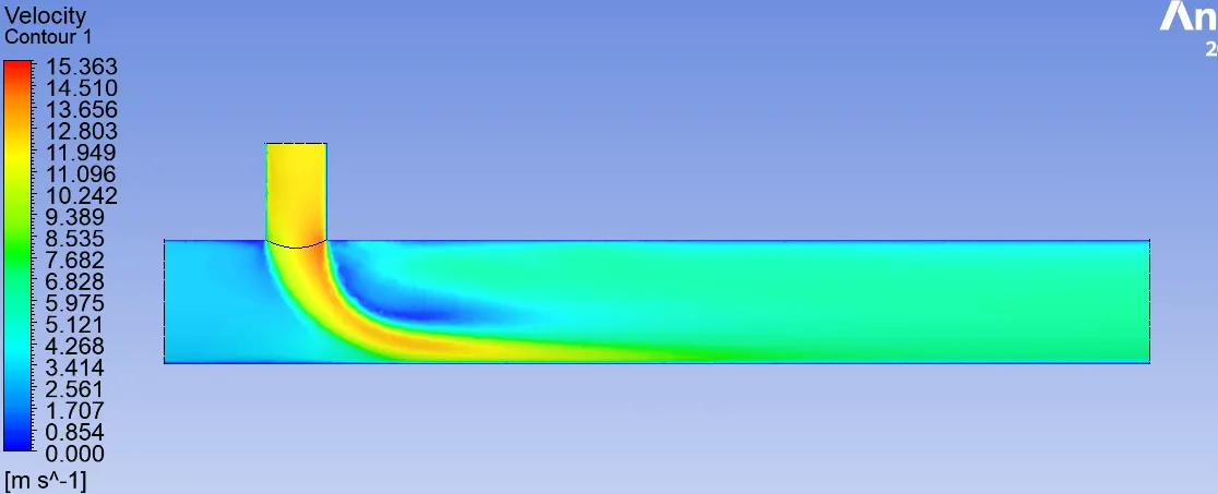
Velocity Contors

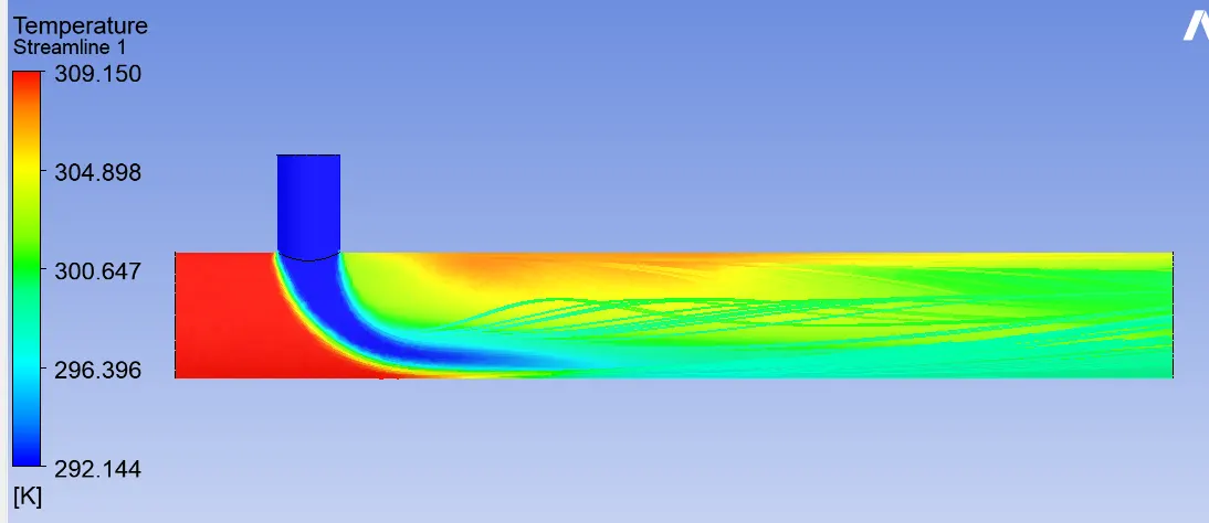
Temperature Streamline

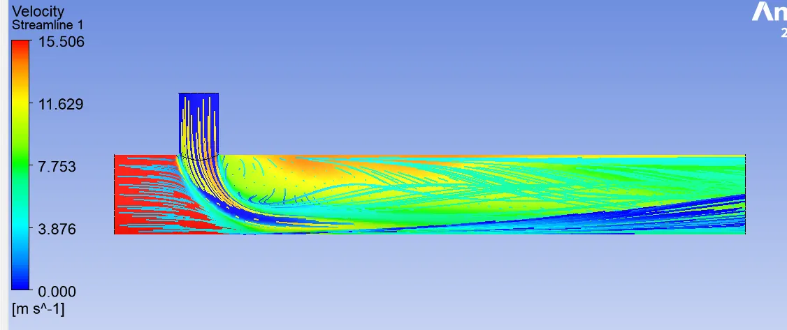
Velocity Streamline

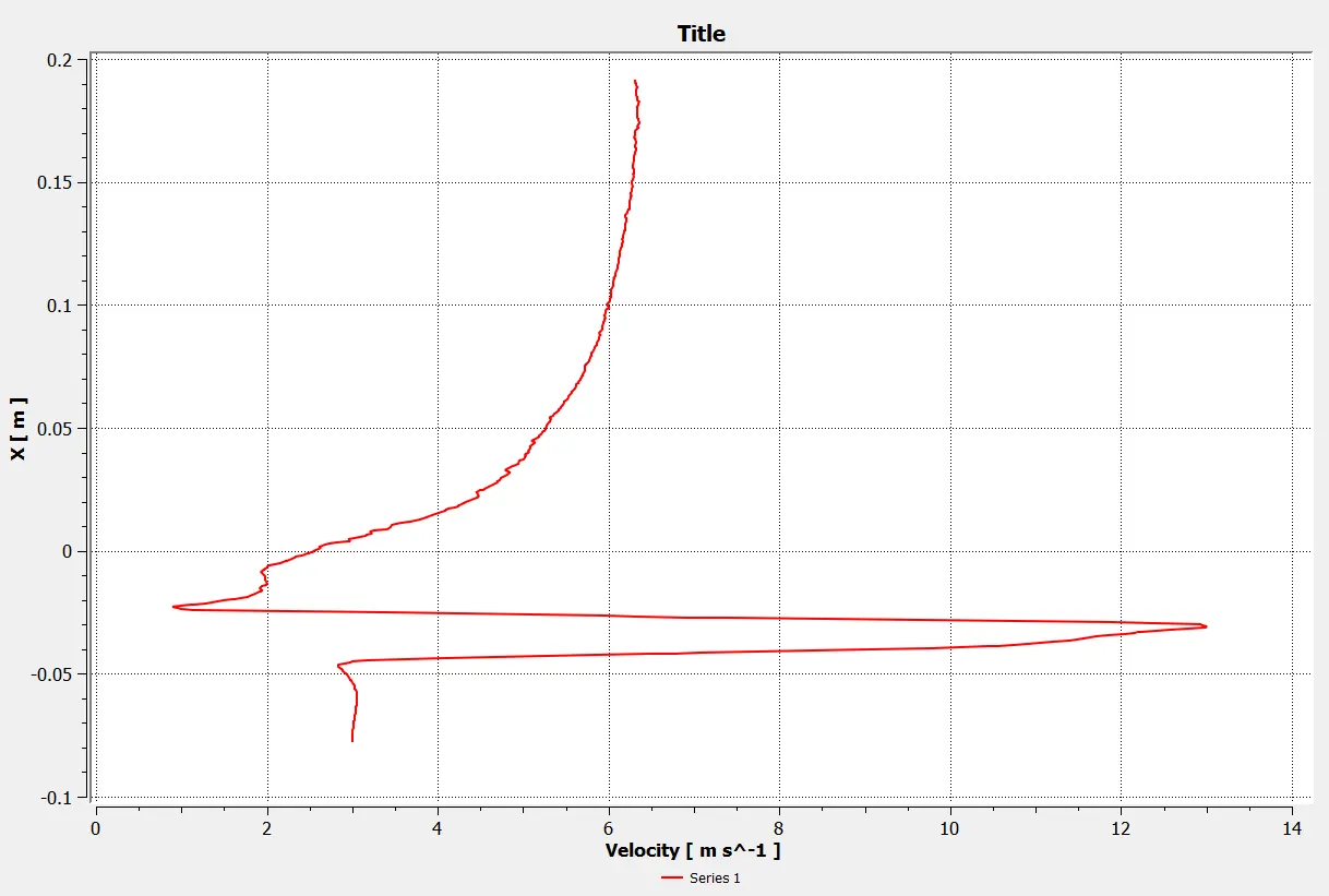
velocity and temperature line Plots

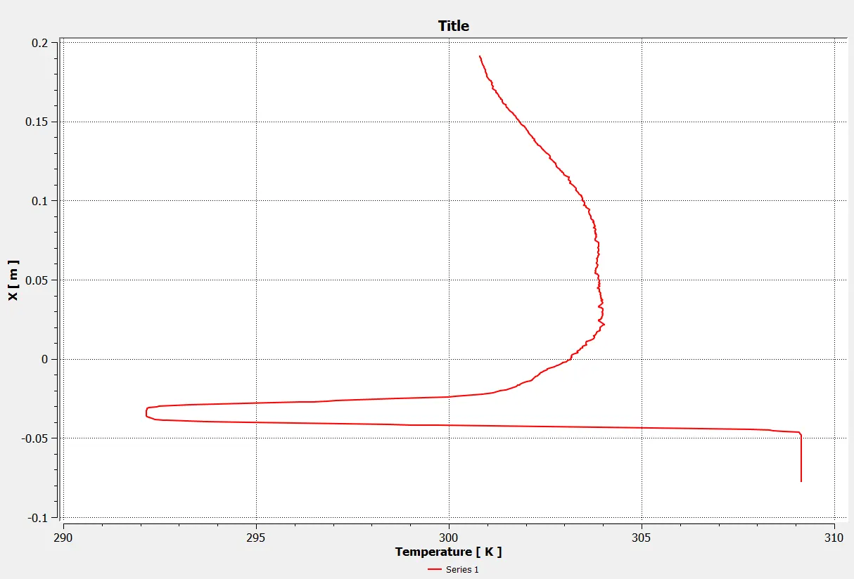
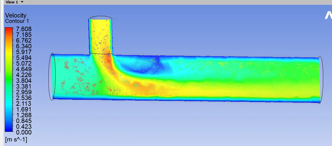
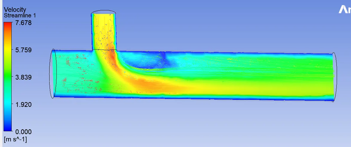
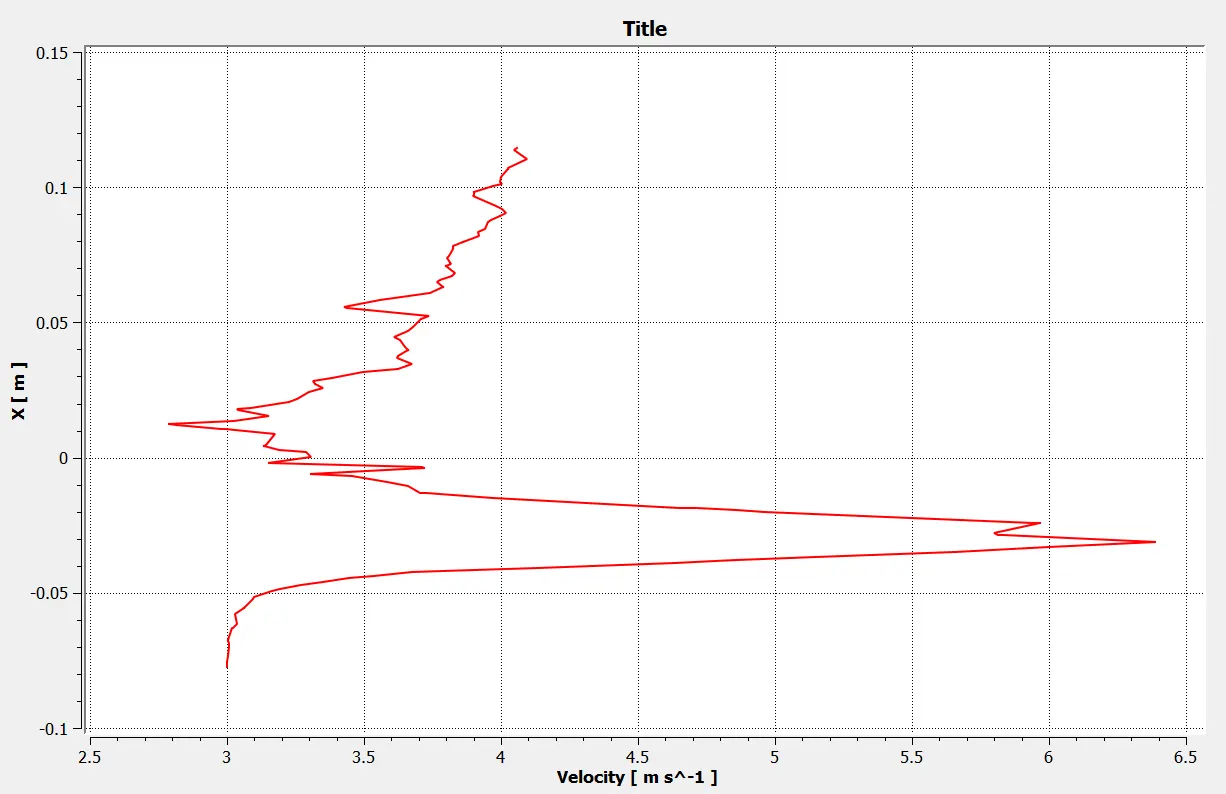
Mesh independent study case1

short Mixing Tee:

Inlet velocity-3m/s

Momentum ratio-2

Converge Plot:

The solution is converge into 150 iteration.

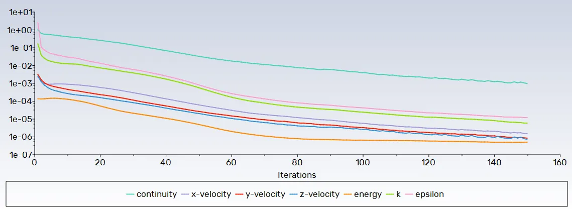
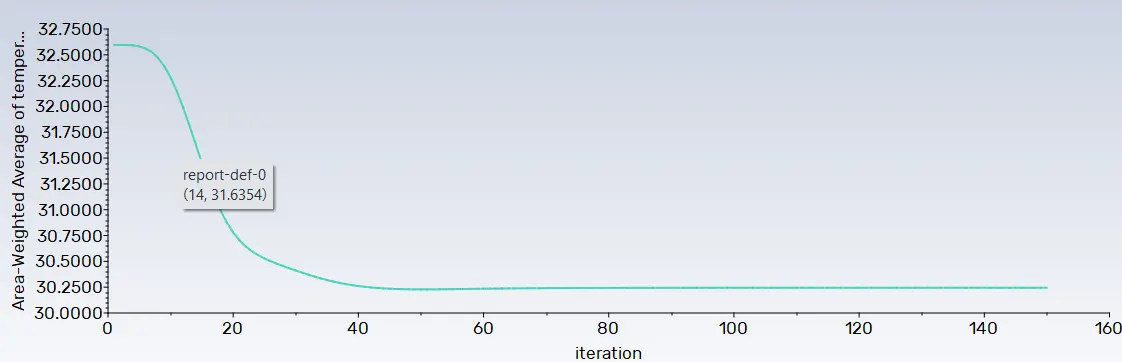
 Area-Weight Average of temperature

The average temperature at outlet is 30.2568C

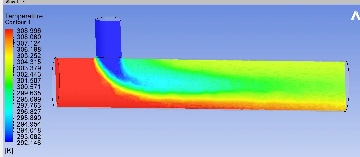
Temperature contours

Velocity Contours

Temperature streamline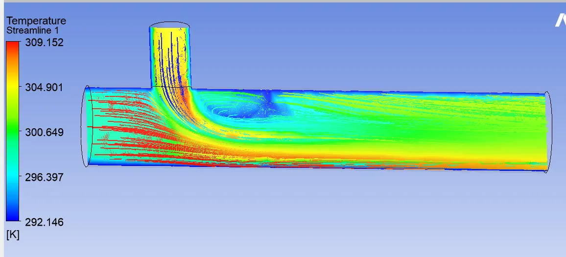

Velocity Streamline

Velocity and temperatue line plots

                 MR     Element      Node          Area weight average       Converge         temperature      Velocity

short pipe   2        576190         110523           30.39080                      125              309.150          8.591

short pipe   4        576190         110523            27.54950                    198              308.996          14.970               

Long pipe    2        765897         147068            30.46780                    119               308.996         8.707

Long pipe    4        765897         147068           27.28760                     156                308.994        15.363

• View the table in the short and long mixing tee to the momentum ratio change to undrstand the how the temperature and Velocity change in the mixing tee.In the case 1 in short mixing tee to take same length and change the hot inlet velocites are same  and cold inlet velocites chane wwith repect to momentum ratio.To understand the turblent mixing at the tee joint betwwn hot air and cold air because of high velocity of cold air,Which is not possible in case of low-velocity cold air.
• The temperature contour at the outlet for short tee cases shows that some of the high temperatures flow sips through without properly mixing with the flow. Whereas, in the temperature contour of long tee cases, the high temperatures flow thoroughly mixes with the rest of the flow.Therefore, we can recommend using the long tee and high-velocity inlet for application. This is because we have a area -weight average in the case of long tee compared to the short tee for both momentum ratios.

Conclusion:

• after seen in Case-1-a and Case-1-b, the temperature at the outlet drops down significantly due to the high velocity of cold air from the inlet. This is possible due to the turbulent mixing at the tee joint between hot air and cold air because of the high velocity of cold air., which is not possible in the case of low-velocity cold air.
• The temperature contour at the outlet for short tee cases shows that some of the high temperatures flow sips through without properly mixing with the flow. Whereas, in the temperature contour of long tee cases, the high temperatures flow thoroughly mixes with the rest of the flow.
• Therefore, we can recommend using the long tee and high-velocity inlet for application. This is because we have a area -weight average in the case of long tee compared to the short tee for both momentum ratios.
• k- epsilon model predicts away from boundaries (wall) and k- omega model predicts near the wall. Therefore, the K-epsilon model is majorly used for free flow away from the wall and as in this project, there is no dealing with the wall of the mixing tee for change in temperature along the length of it, so the K-epsilon model was chosen for further .