Week 1- Mixing Tee

Objective :

1) To set up steady-state simulations to compare the mixing effectiveness when hot inlet temperature is 36⁰C & the Cold inlet is at 19⁰C for 2 given models .

2) To compare the results while using k-omega sst and k-epsilon for first model and hence use most suited method for further calculations .

3) Set up the cases as per given requirememnts .

1. Case 1
   • Short mixing tee with a hot inlet velocity of 3m/s.
   • Momentum ratio of 2, 4.
2. Case 2
   • Long mixing tee with a hot inlet velocity of 3m/s.
   • Momentum ratio of 2, 4.

4) Compare the following values for each cases

1. Cell count
2. Average outlet temperature
3. Number of iterations for convergence

5) Plot graphs and contours and explain the following

1. Velocity and temperature contour plots on the cut planes along and across the pipe.
2. Velocity and temperature line plots along and across the length of the pipe.
3. Perform Mesh independent study for any one case.
4. Discuss the effect of length and momentum ratio on results.

Procedure :

The procedure for all cases are same , hence the set up for one case will be explained .

Step 1: Open ansys workbench

step 2: Drag and drop fluid flow (fluent) analysis system to the project schematic box .

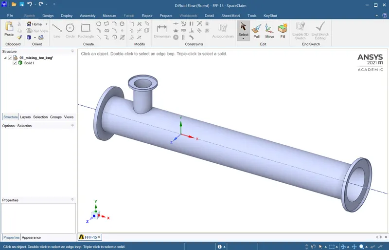
step 3: Open the geometry module and import the given solid model into the space claim interface .

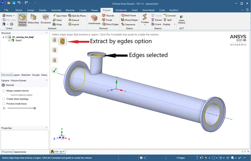
step 4: Go to prepare option > select the volume extract option > select extract by edges option > click on the edges to be extraced and click on tick option to extract the required volume .

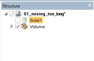
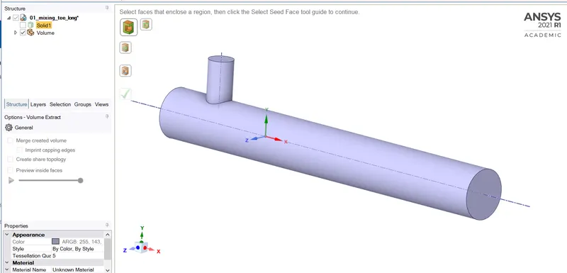
Step 5: De-select the solid option from structure tab > right clich on solid component and click on supress for physics option . Hence we have obtianed the model for solving. Close the geomtery module > Right click on geometry module and click on update option .

Step 6: Open Mesh module .

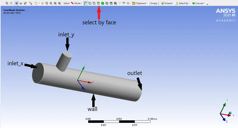
Click on select by face option> select respective faces and name them according to required set up .

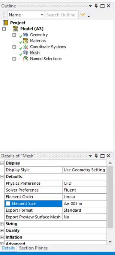
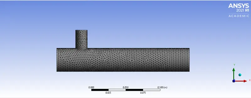
Step 7: Click on mesh tab> select defaut option> enter required mesh size> right click on mesh tab and click on generate mesh to obtain a mesh . Close the mesh module > Right click on mesh module and click on update .

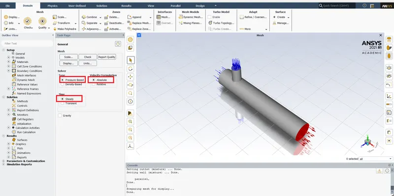
Step 8: Open the set up module . Ensure the required type of solver has been selected .

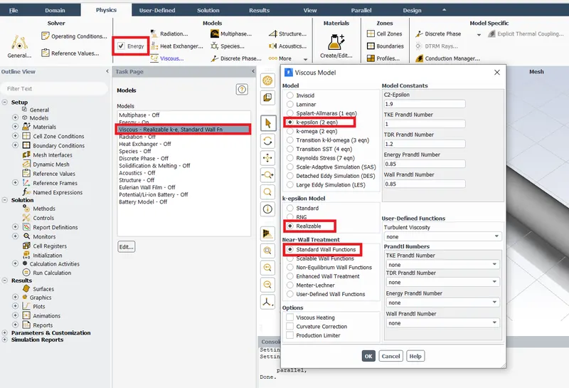
Step 9: Click on energy option in model tab > select the required viscous model > select the model type as k-epsilon >realizable with standard wall functions.

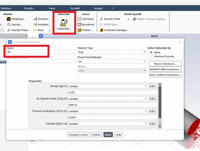
Step 10 : Click on materials option and select the working fluid (air in this case)

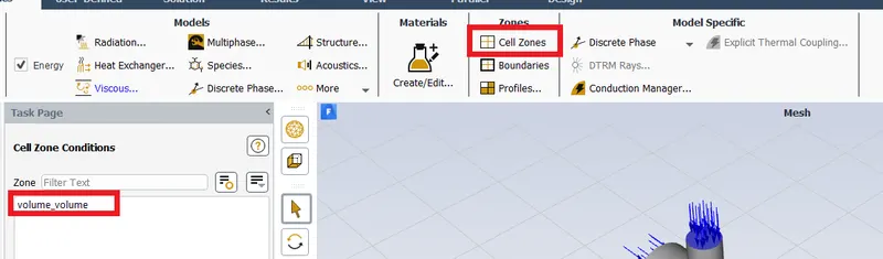
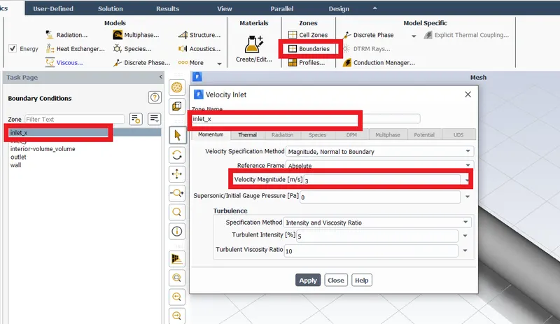
Step 11 : Click on cell zones > select the vloume required . Click on boundary option > Input required boundary conditions for each face required .

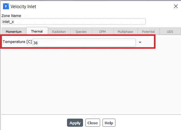
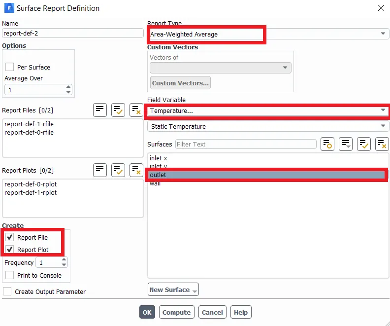
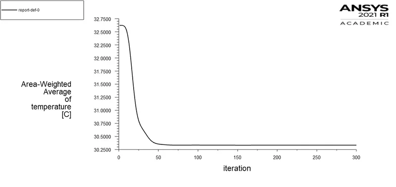
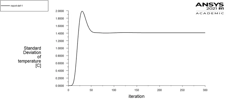
Step 12: Click on solutions tab > definitions>new > surface report > area weighted average > select required variable and face . Then click on initialize > input number of iterations > calculate .

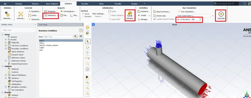
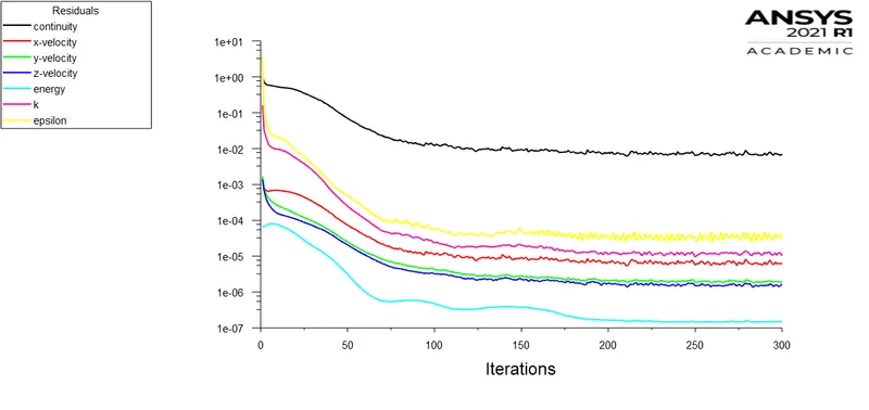
Step 13: Now we have made set up for processing the problem .We shall obtain plots for standard deviation , area weighted average, scaled residuals etc once the solver has run . Now close the set up module . Open Results for post processing .

Outputs :

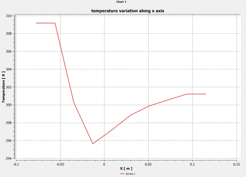
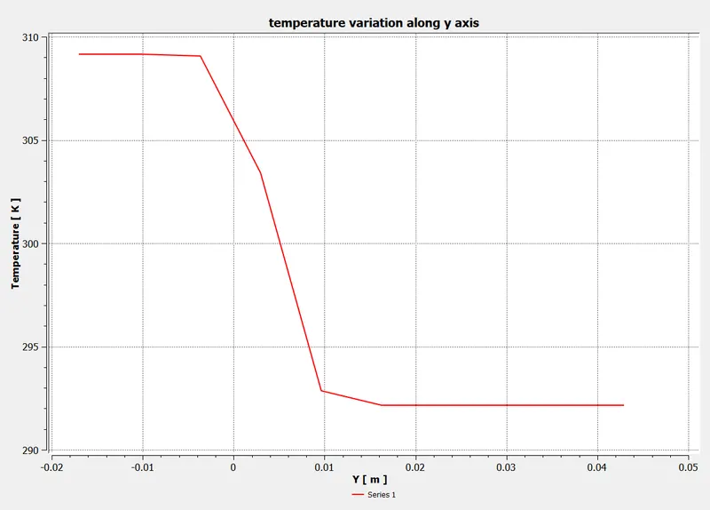
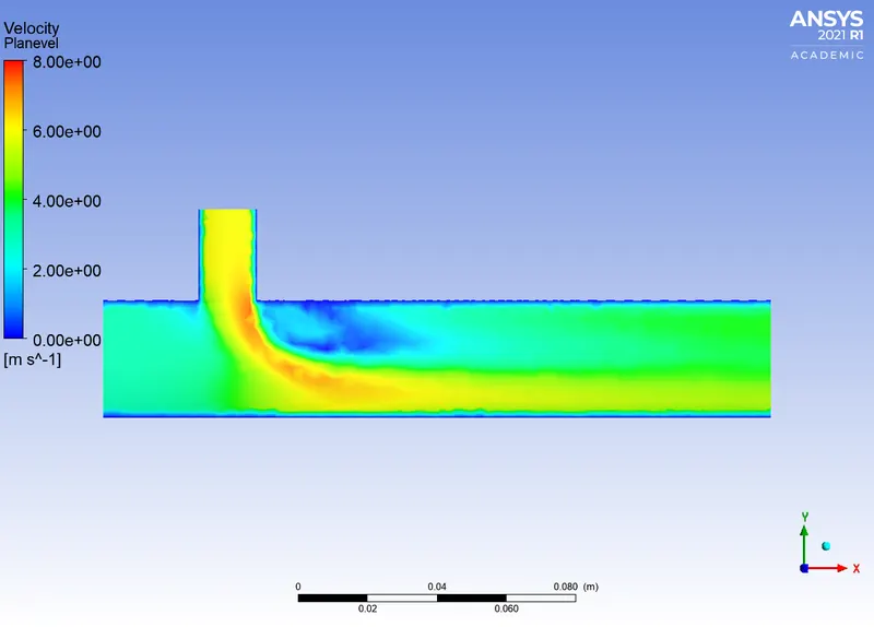
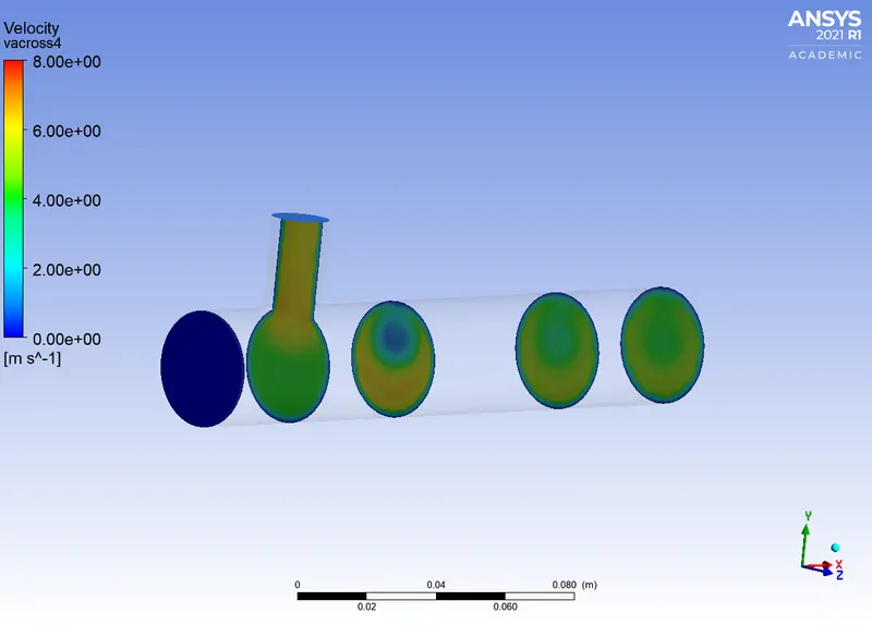
Case 1 a : Short tee

Hot inlet velocity = 3m/s

Momentum ratio =2

Cold inlet velocity = 6m/s.

Model type : k-epsilon

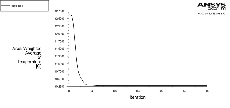
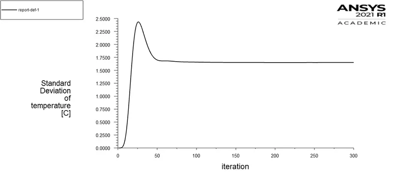
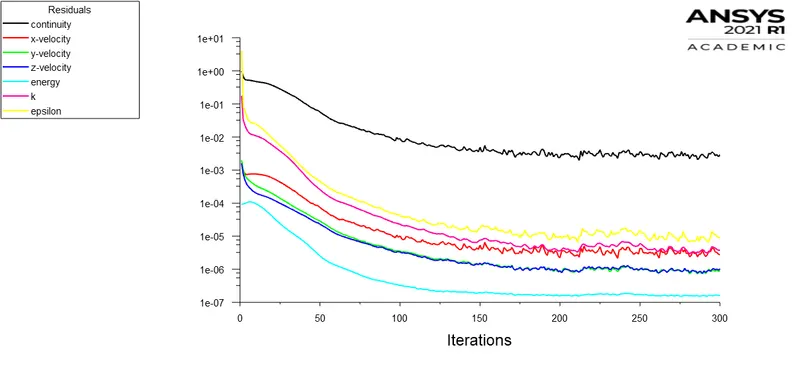
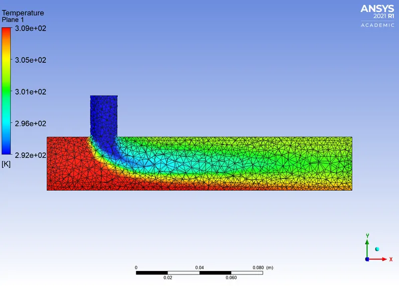
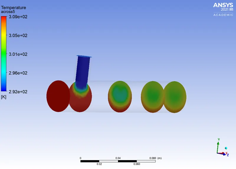
Temperature contours and plots along and across the pipe

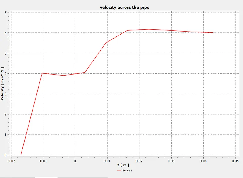
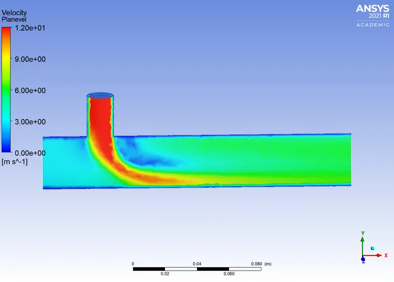
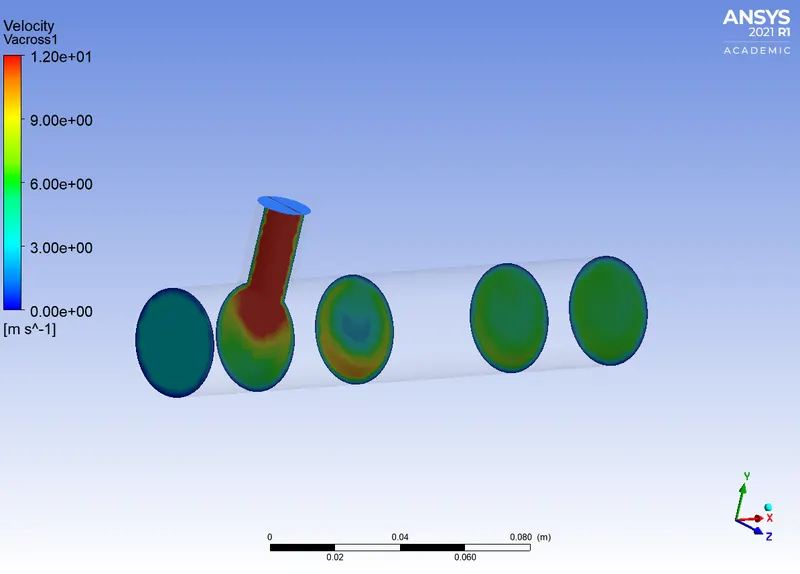
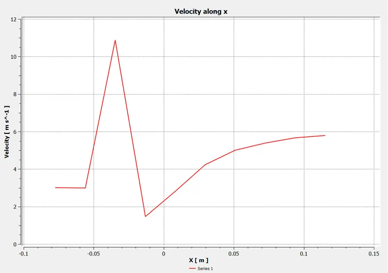
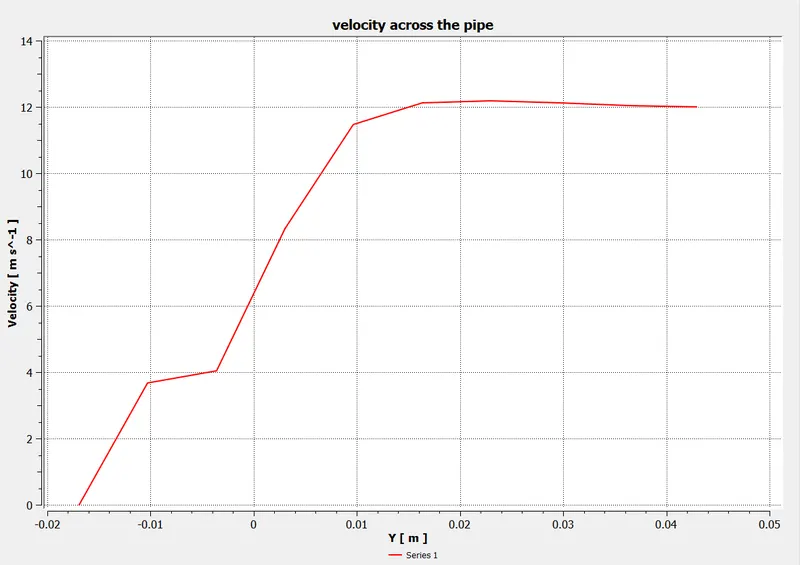
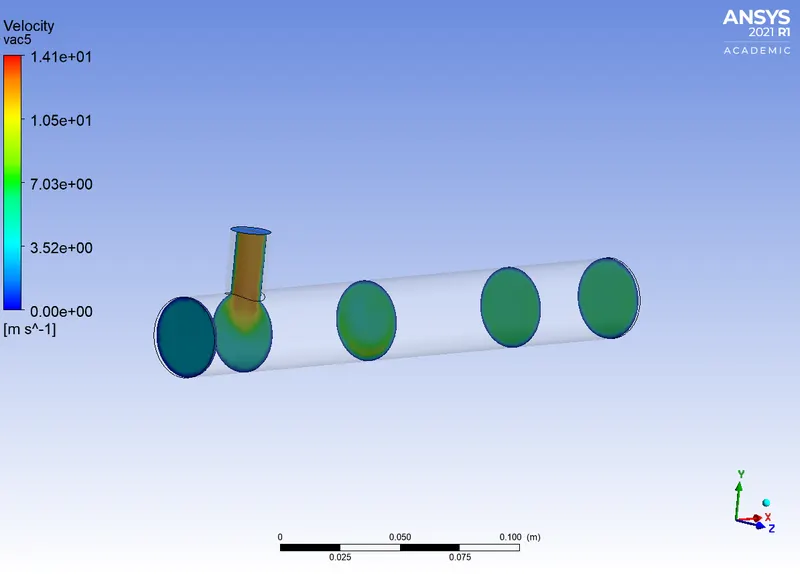
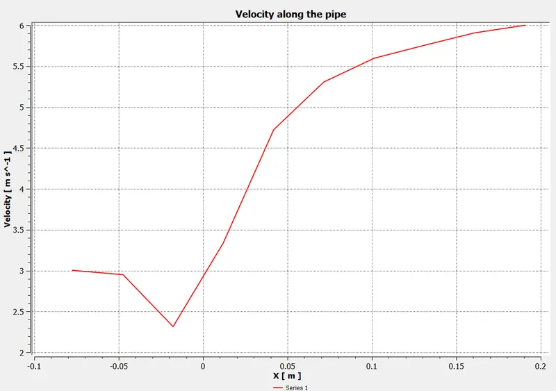
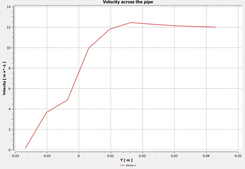
Velocity contours and plots along and across the pipe

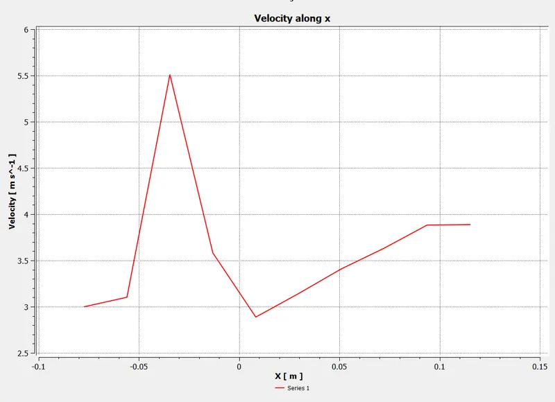
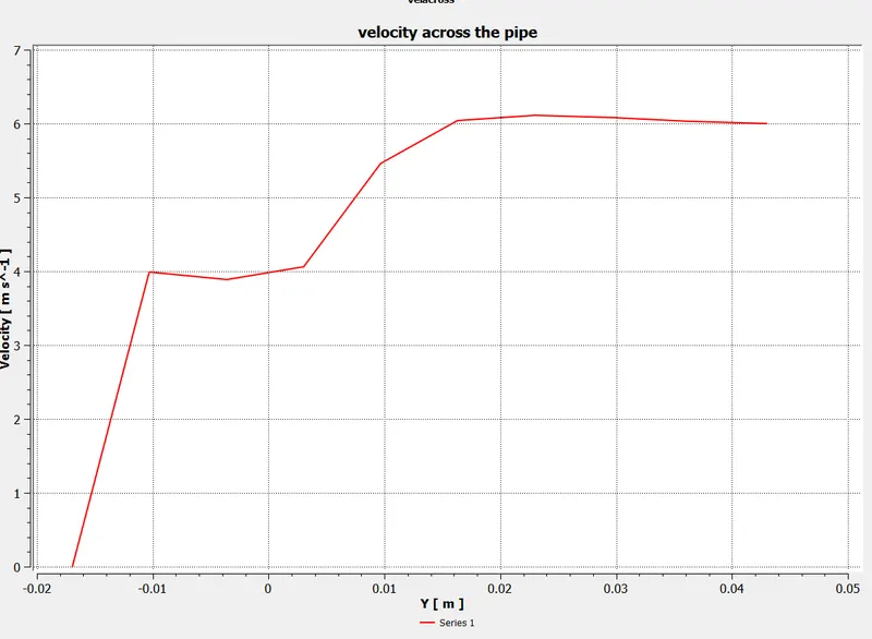
Case 1 b : short tee

Hot inlet velocity = 3m/s

Momentum ratio =2

Cold inlet velocity = 6m/s.

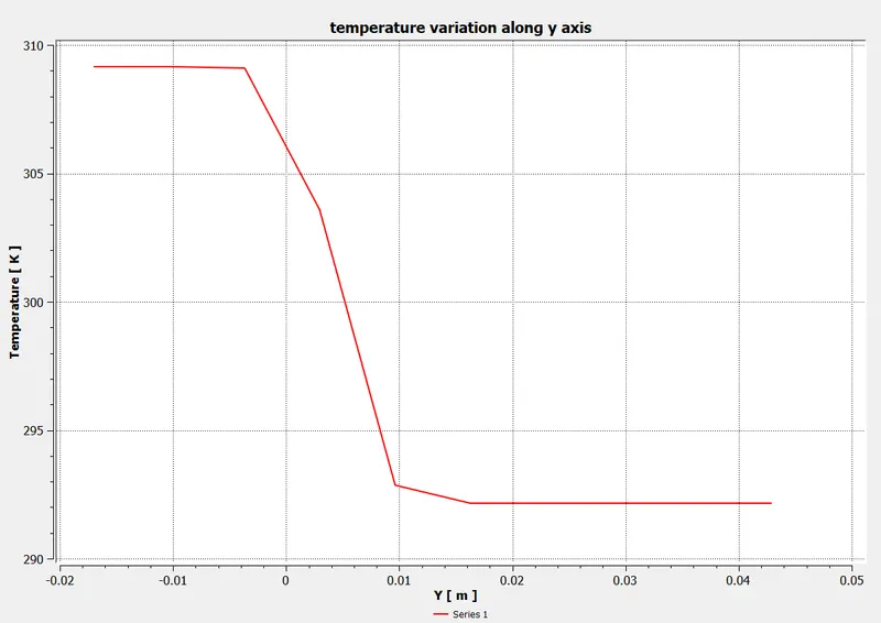
Model type : k-omega sst

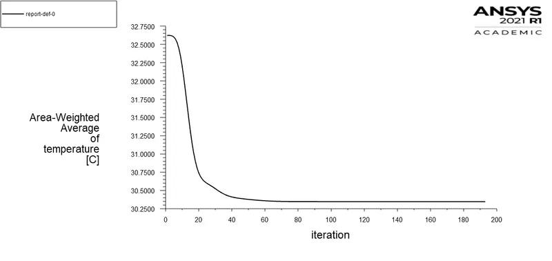
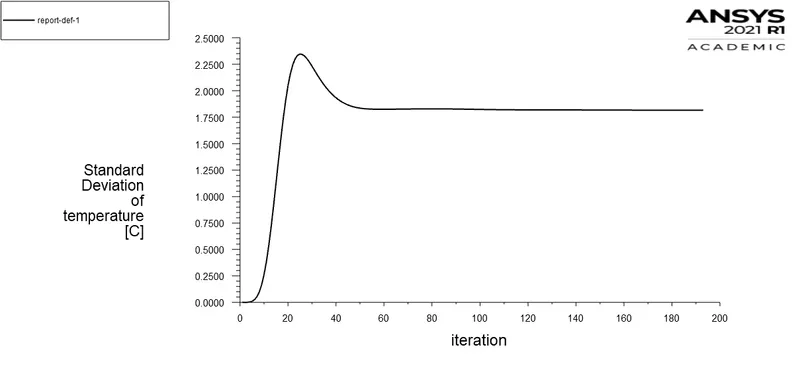
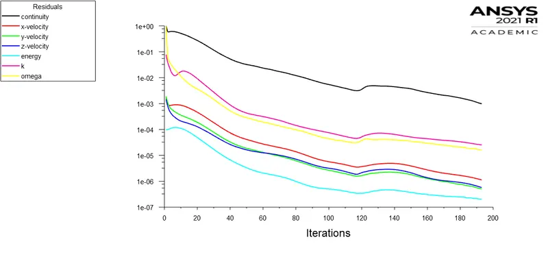
temperature contours and plots along and across the pipe

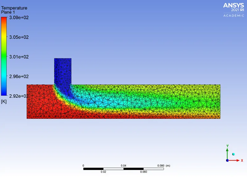
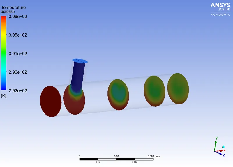
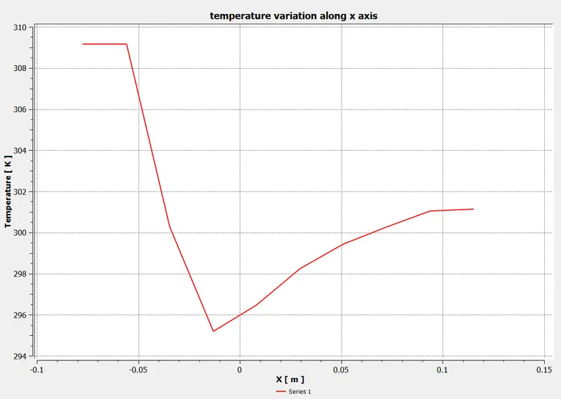
Velocity contours and plots along and across the pipe .

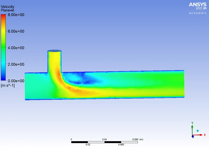
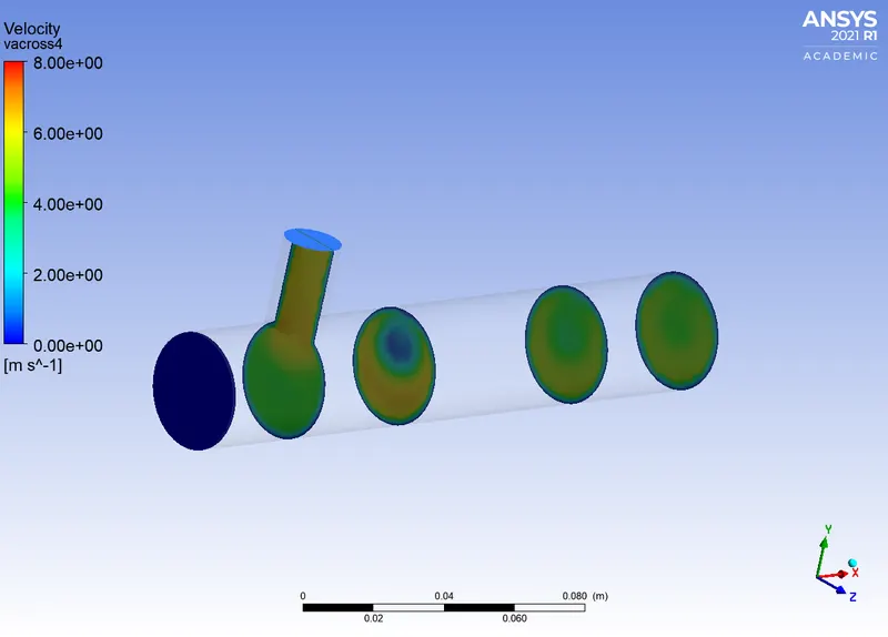
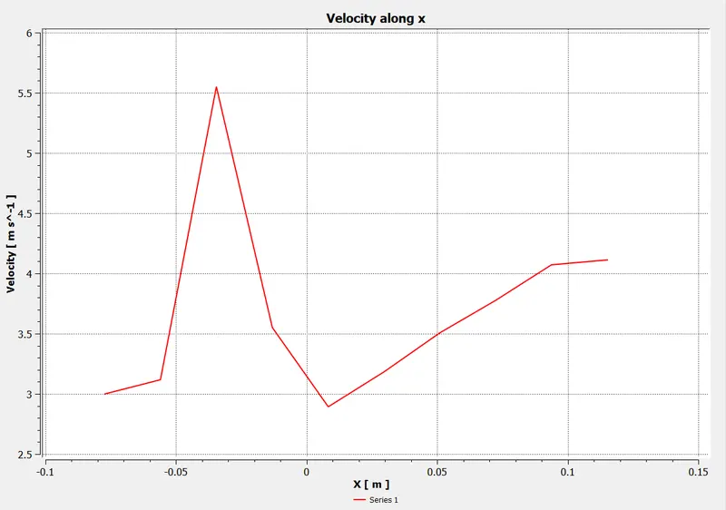
k- epsilon model predicts well far from the boundaries (wall) and k-omega model predicts well near wall . The solution has converged at 175 Iterations for k-epsilon and 192 Iterations for k-omega . In this case , since our studies are not neat the boundaries, we shall use k-epsilon for further cases .

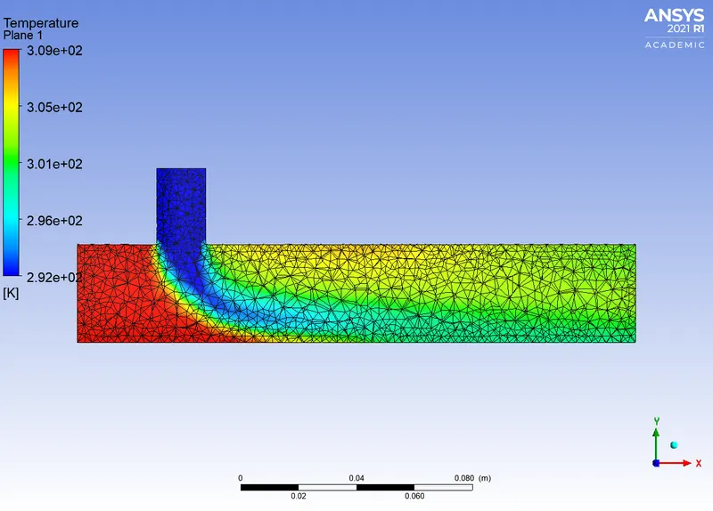
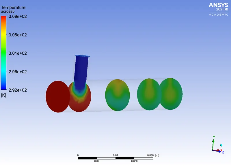
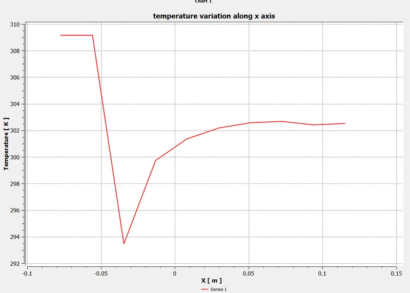
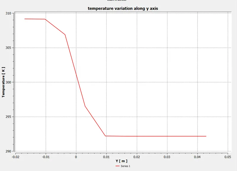
Case 1 c: Short tee

Hot inlet velocity = 3m/s

Momentum ratio =4

Cold inlet velocity = 12m/s.

Model type : k-epsilon

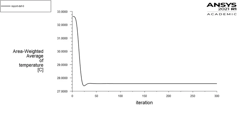
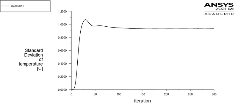
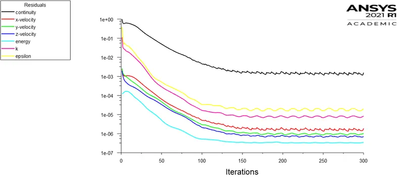
Temperature contours and plots along and across the pipe

Velocity contours and plots along and across the pipe .

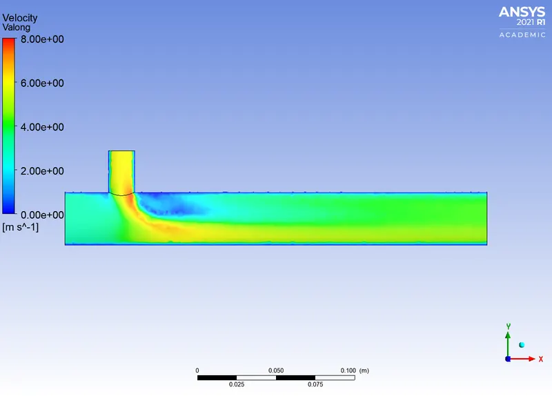
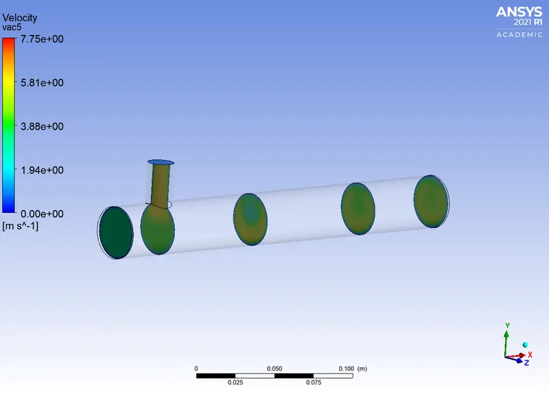
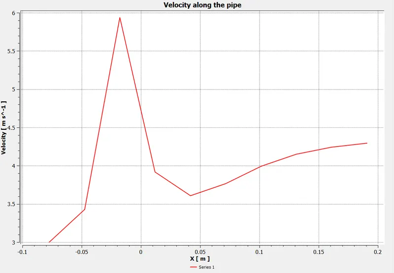
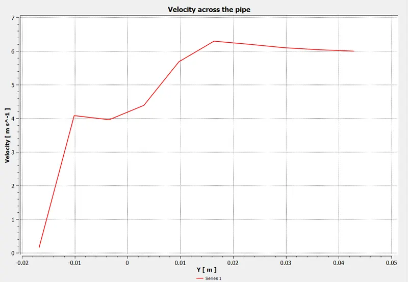
Case 2 a : Long tee

Hot inlet velocity = 3m/s

Momentum ratio =2

Cold inlet velocity = 6m/s.

Model type : k-epsilon

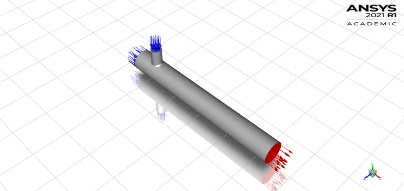
Model image

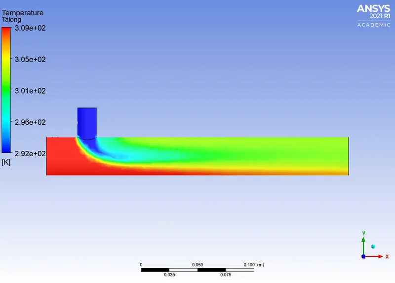
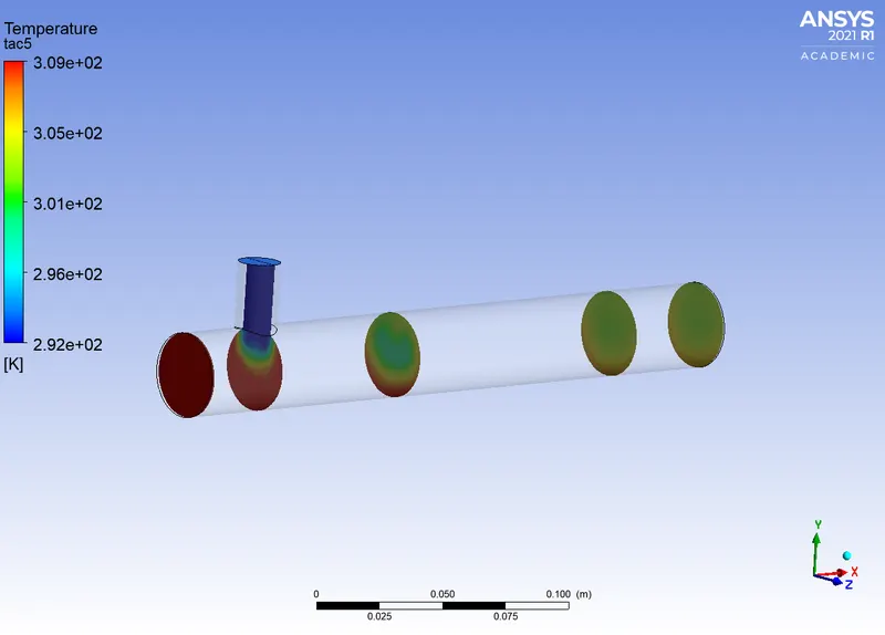
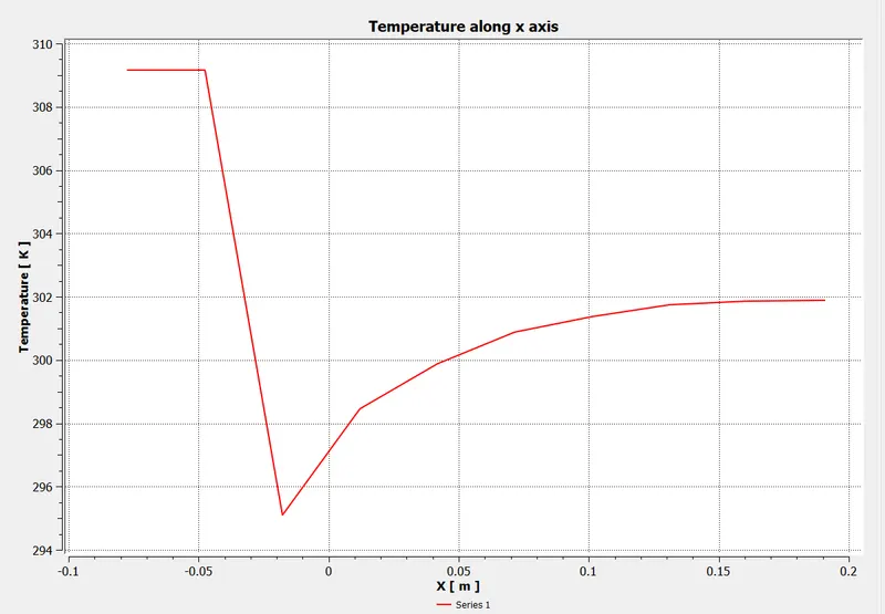
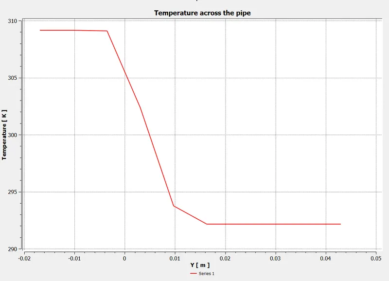
Temperature contours and plots along and across the pipe

Velocity contours and plot along and across the pipe

Case 2 b: Long tee

Hot inlet velocity = 3m/s

Momentum ratio =4

Cold inlet velocity = 12m/s.

Model type : k-epsilon

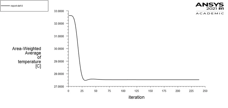
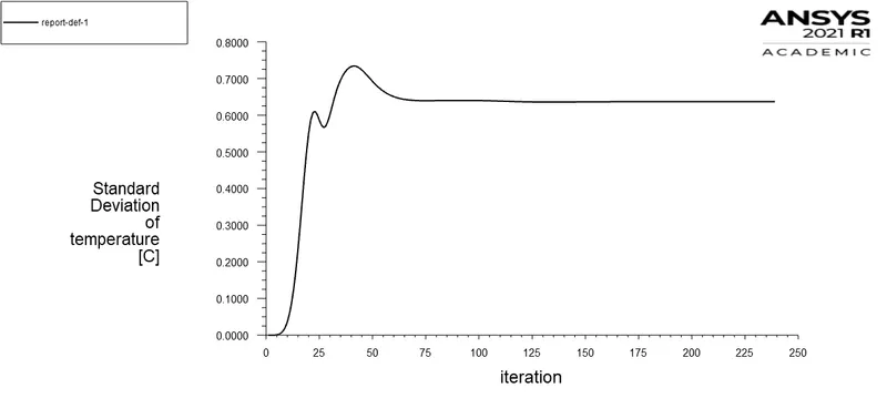
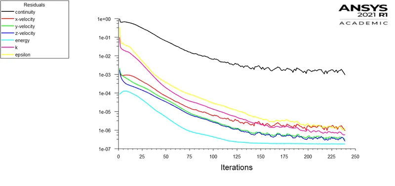
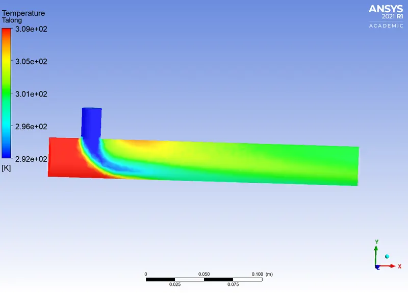
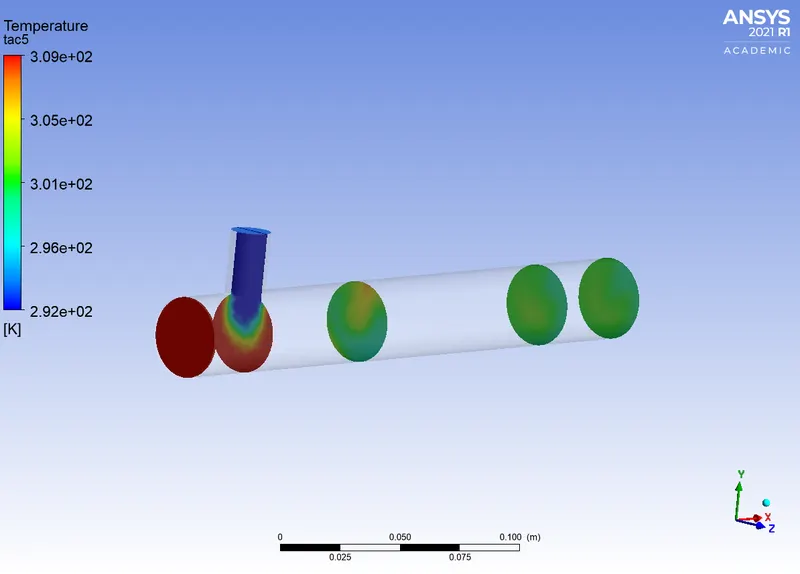
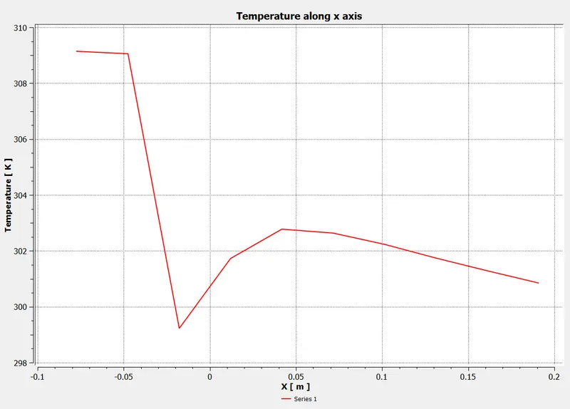
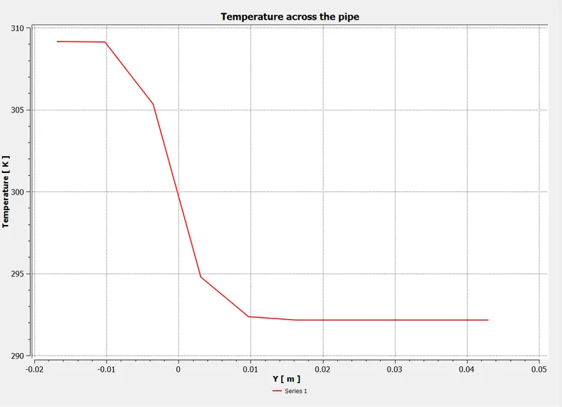
Temperature contours and plot along and across the pipe

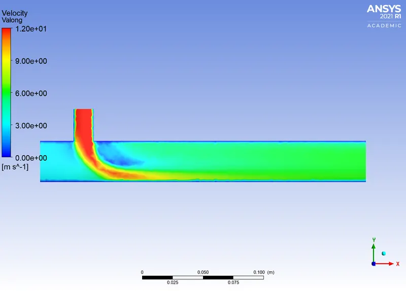
Velocity contours and plot along and across the pipe

Results :

1)

Analytical Solution

m = `rho * A*V`

Area of cold inlet: .0002 `m^2`

Area of hot inlet : .0009 `m^2`

`m_(hot) = rho_(air)*A_(hot).V_(hot)` `

rho_air at 19 degree=1.225kg/m^3

rho air at 35 degree = 1.145 kg/m^3

case 1: momentum ratio = 2

V_hot= 3m/s

V_cold=6m/s

m_hot = 1.145*.0009*3 =0.0030915

``m_(cold) = rho_(air)*A_(cold).V_(cold)``

m_cold= 1.225*.0002*6=0.00147

T_mixture=30.52 degree celcius

Case 2: Momentum ratio =4

m_hot = 1.145*.0009*3 =0.0030915

m_cold= 1.225*.0002*12=.00294

T_mixture=27.71 degree celcius

Sl no	CASE	Cell count	Average outlet temperatue	Number of iterations for convergence
1	CASE 1a :Short tee Hot inlet V=3m/s Cold inlet V=6m/s	39879	30.273	175
2	CASE 1b: Short tee Hot inlet V=3m/s Cold inlet V=6m/s	39879	30.347	192
3	CASE 1c: Short tee Hot inlet V=3m/s Cold inlet V=12m/s	39879	27.567	150
4	CASE 2a: Long tee Hot inlet V=3m/s Cold inlet V=6m/s	56360	30.334	200
5	CASE 2: Long tee Hot inlet V=3m/s Cold inlet V=12m/s	56360	27.531	175

2) To study mesh independence , Case 1 a was solved using 3 mesh sizes

The table below shows cell count, element length and average temperature output for all the 3 cases .

Sl no	Element Length	Cell Count	Average temperature
Case 1 a i	.003 m	39879	30.273
Case 1 a ii	.005 m	14228	30.215
Case 1 a iii	.01 m	12728	30.217

Here we can observe that the output does not vary significantly for all the 3 cases , hence we can conclude that mesh independence has been obtained at .01m element length .

3)

Length : From the outputs , we can observe that , as length increases , the number of iterations to converge also increases

Momentum Ratio : We can observe that , as momentum raio increases , the rate of diffussion increases, hence the iterations to conververge decreases.