Week 1- Mixing Tee

AIM: 1. To set up steady-state simulations to compare the mixing effectiveness when hot inlet temperature is 36⁰C & the Cold inlet is at 19⁰C.

• Case 1:

Short mixing tee with a hot inlet velocity of 3m/s.

Momentum ratio of 2, 4.

• Case 2:

Long mixing tee with a hot inlet velocity of 3m/s.

Momentum ratio of 2, 4.

2. To view the results along and across the pipe for velocity and temperature contour and line plots.
3. To compare the results in a table and discuss it in conclusion.

INTRODUCTION:

The function of mixing Tee is to provide proper mixing of quantities to get the desired result at the outlet. By controlling the velocity of chilled air, we can get the desired temperature in the room.

CFD simulations can provide accurate predictions of the mixing behaviour including temperature and velocity, etc.

SOLVING & MODELLING APPROACH:

GEOMETRY: Construct a two- or three-dimensional representation of the object to be modelled and tested using the work plane coordinate system within ANSYS.

MESH: At this point ANSYS understands the makeup of the part. Now define how the modelled system should be broken down into finite pieces.

SETUP: The case setup will be done using Ansys fluent

SOLUTION: Ansys fluent where run time result visualization is done

RESULTS: Post processing of results will be done here using CFD-post

GEOMETRY SETUP:

• The computational models are uploaded to the Ansys Space Claim as a step file.
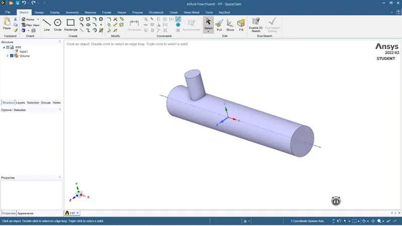
• For this assignment, we are interested in performing fluid flow analysis through the geometry, hence we used the volume extraction option to extract the fluid volume from the geometry

PROCEDURE:

• Open Ansys fluent workbench.
• Open new spaceclaim geometry.
• Open files and import and the short mixing tee geometry.
• Go to prepare > volume extract > select face enclosure region > select the faces > Click on seed select > select any one of the inlet face > ok.
• The volume will be created and the shell can be suppressed to physics and disable the shell.
• Now the save the file as spaceclaim doc.
• Go to geometry > Replace the geometry > Open the saved spaceclaim geometry > Update.
• Repeat the same process for long mixing tee.

FIG 1. Volume Extracted from the given Geometry

MESH GENERATION:

• Open mesh, check the units and click on generate mesh.
• After mesh generation the mesh is not satisfying, so change the mesh type into quad & element size into 2mm.
• Now click on generate.
• Then click on the surface select and select the surfaces to create named selections such as inlet-x, inlet-y & outlet.
• Now close and update the mesh workbench.
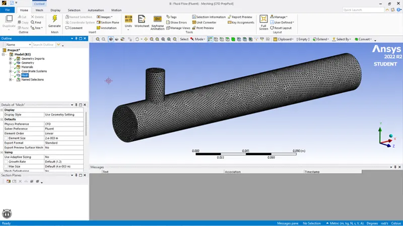
• Repeat the same process for long mixing tee.

FIG 2. Naming the Boundaries

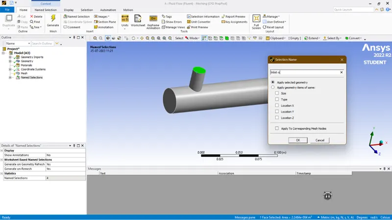
FIG 3. Meshing done for the short tee with mesh length of 2mm

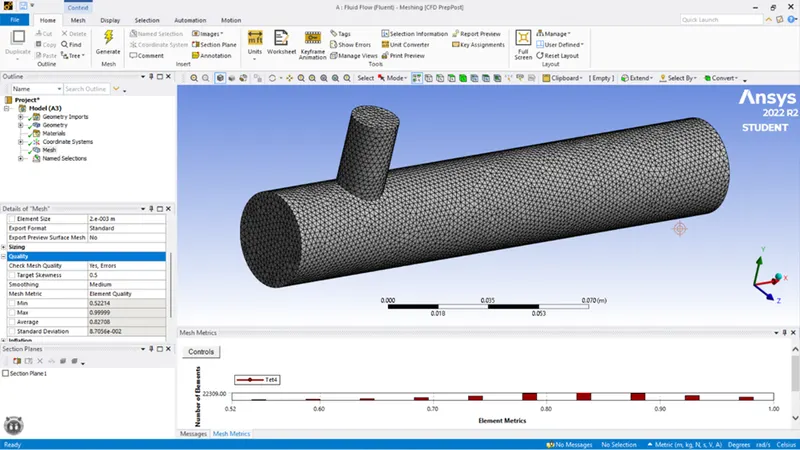
FIG 4. Meshing done for the long tee with mesh length of 2mm

SOLVER SETUP:

1. CASE-1 (short Mixing Tee)

• Solver- steady state.
• Turn on- energy equation (since we need temperature0.
• Turbulence model- laminar (we can also use K-epsilon).
• Boundary conditions > Inlet-x(edit) > Velocity inlet > Variable-temperature > Inlet-x temperature(36degrees) > Inlet-y (19degrees) > Ok.
• Give the "inlet velocity of Inlet-x as 3m/s & Inlet-y as 6m/s".
• Go to solution > create surface report definition > Area weighted average report > Give it a title > Change field variable into - Temperature > Ok.
• Repeat the same process in solution for velocity also.
• Click on Initialize.
• Give the number of iterations as 250 and click on calculate.
• Close the solver.

CASE 1.1:

• Short mixing Tee with a hot inlet velocity of 3m/s.
• Momentum ratio 2.

RESULTS: Shown below

FIG 5. Convergence results

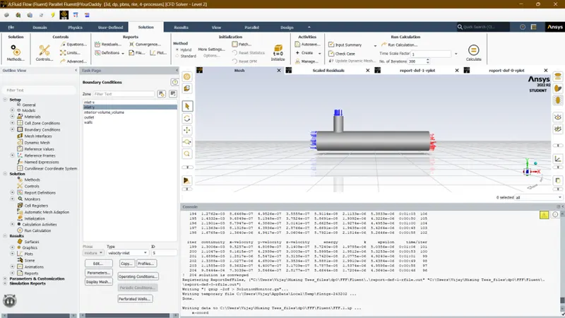
• The solution was converged on 204

FIG 6. Residual plot

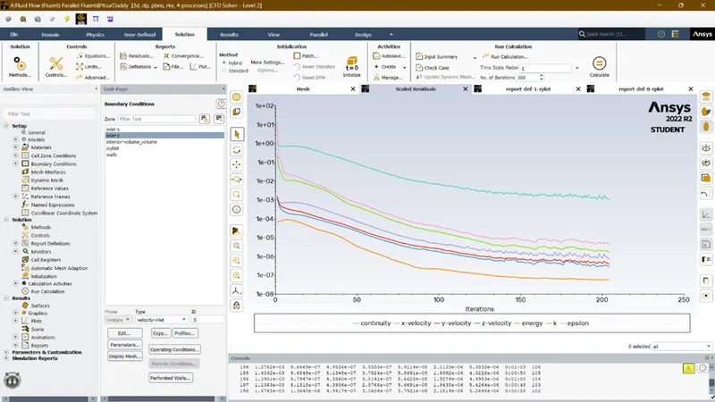
FIG 7. Standard Deviation

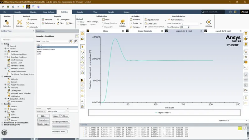
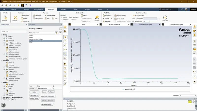
FIG 8. Tavg

CASE 1.2:

• Short mixing Tee with a hot inlet velocity of 3m/s.
• Momentum ratio 4.

SETUP:

• Boundary conditions > Inlet-x(edit) > Velocity inlet > Variable-temperature > Inlet-x temperature(36degrees) > Inlet-y (19degrees) > Ok.
• Give the “inlet velocity of Inlet-x as 3m/s & Inlet-y as 12m/s”.

RESULTS: Shown below

• Give the number of iterations as 300 and click on calculate.
• As the result show convergence will occur above 300.

FIG 9. Residual plot

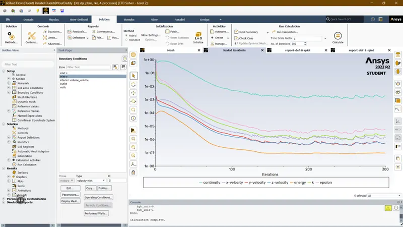
FIG 10. Standard Deviation

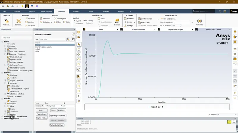
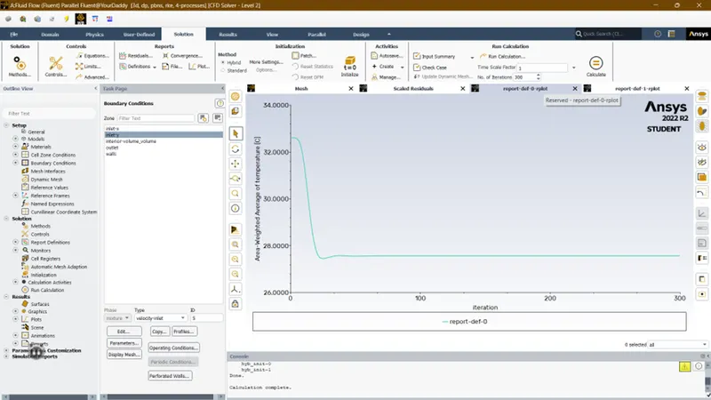
FIG 11. Tavg

CASE-2 (Long Mixing Tee)

• Repeat the same procedure as case 1.

CASE 2.1:

• Long mixing Tee with a hot inlet velocity of 3m/s.
• Momentum ratio 2.

SETUP:

• Boundary conditions > Inlet-x(edit) > Velocity inlet > Variable-temperature > Inlet-x temperature(36degrees) > Inlet-y (19degrees) > Ok.
• Give the “inlet velocity of Inlet-x as 3m/s & Inlet-y as 6m/s”.

Result: Shown below

FIG 12. Convergence Results

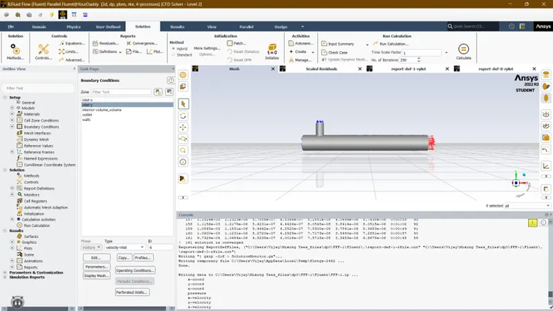
FIG 13. Residual plot

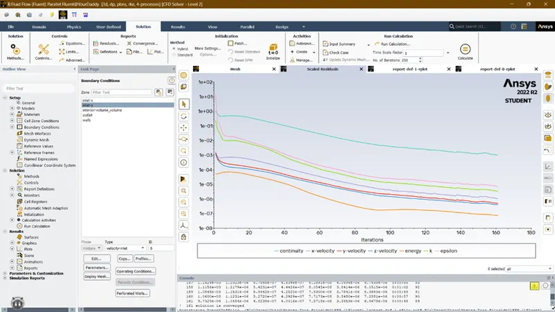
FIG 14. Standard deviation

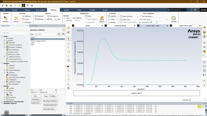
FIG 15. Tavg

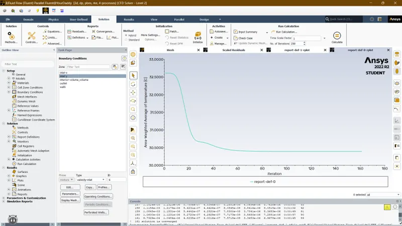
CASE 2.2:

• Long mixing Tee with a hot inlet velocity of 3m/s.
• Momentum ratio 4.

SETUP:

• Boundary conditions > Inlet-x(edit) > Velocity inlet > Variable-temperature > Inlet-x temperature(36degrees) > Inlet-y (19degrees) > Ok.
• Give the “inlet velocity of Inlet-x as 3m/s & Inlet-y as 12m/s”.

RESULT: Shown below

FIG 16. Residual plot

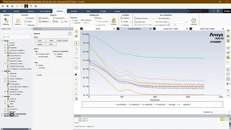
FIG 17. Standard deviation

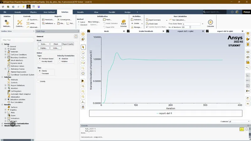
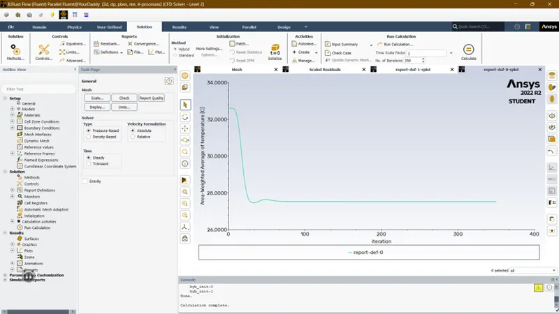
FIG 18. Tavg

POST-PROCESSING:

1. Contours:

• Create a new contour-1 > Change into variables > Temperature > select the volume to display.
• Create contour-2 > variables > velocity > select the volume.
• Create a plane along YZ axis & change the variables to see along and across the pipe by duplicating the plane again and moving it to another location for many views.
• Repeat the process for both the cases.

FIG 19. Temperature of short tee (Case 1.1)

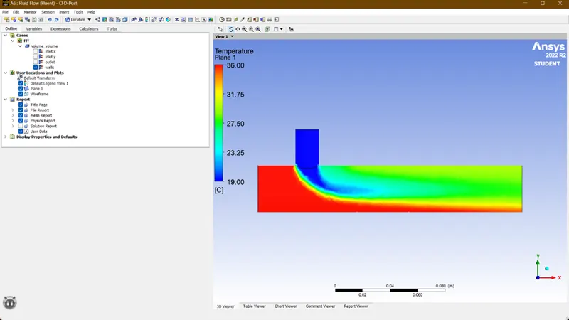
FIG 20. Velocity of short tee (Case 1.1)

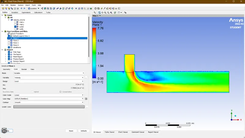
FIG 21. Temperature across the short tee (case 1.1)

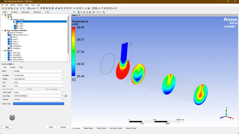
FIG 22. Velocity across the short tee (case 1.1)

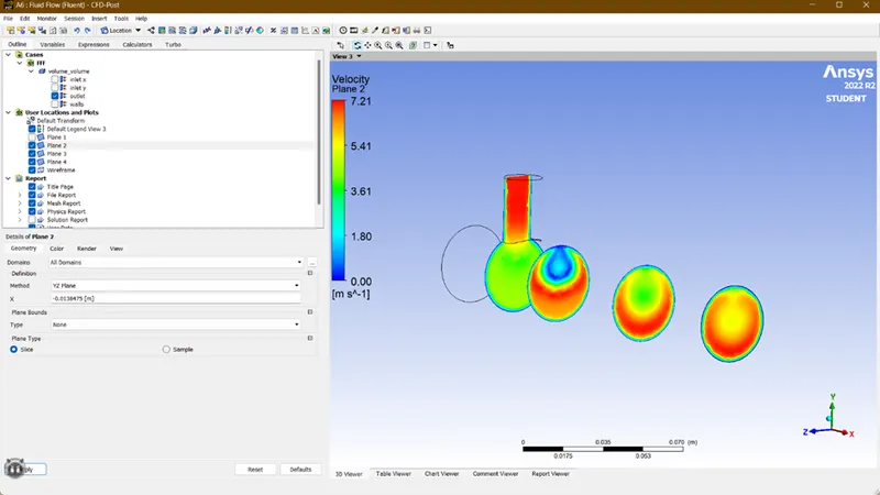
FIG 23. Streamline of Temperature across the short tee (case 1.1)

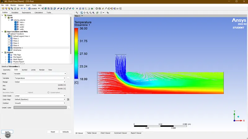
FIG 24. Streamline of Velocity across the short tee (case 1.1)

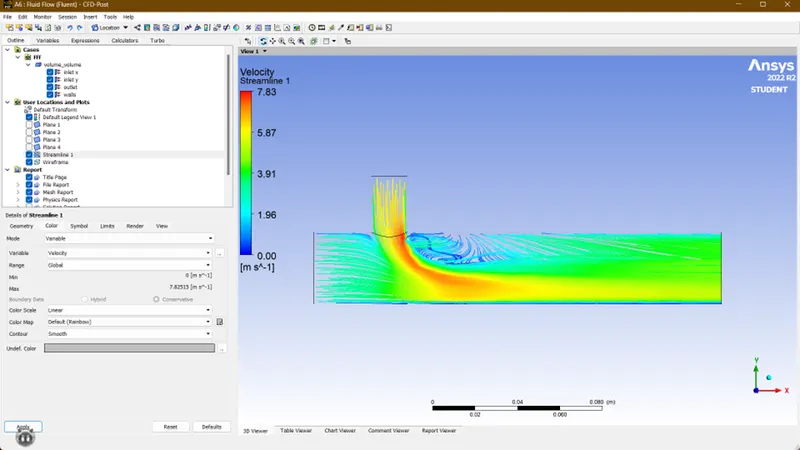
FIG 25. Temperature of short tee (Case 1.2)

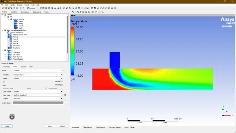
FIG 26. Velocity of short tee (Case 1.2)

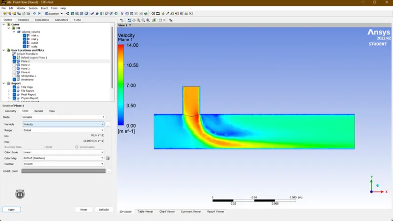
FIG 27. Temperature across the short tee (Case 1.2)

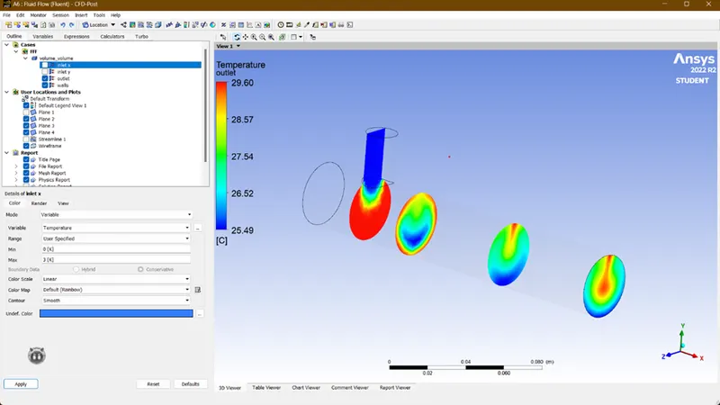
FIG 28. Velocity across the short tee (Case 1.2)

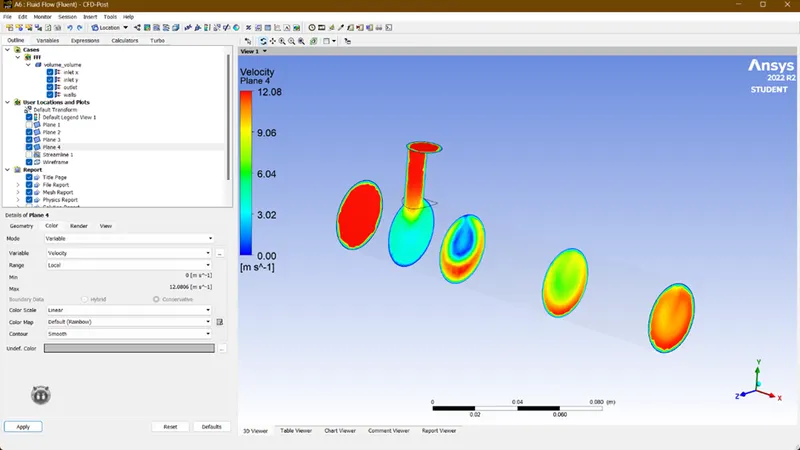
FIG 29. Streamline for Temperature across the short tee (Case 1.2)

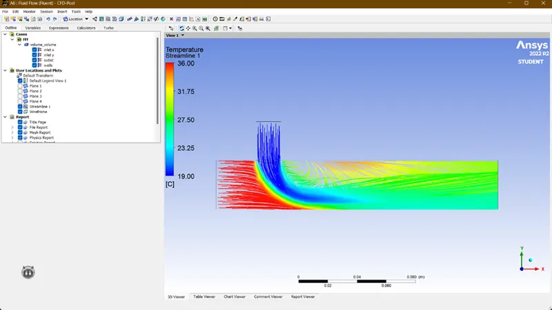
FIG 30. Streamline for Velocity across the short tee (Case 1.2)

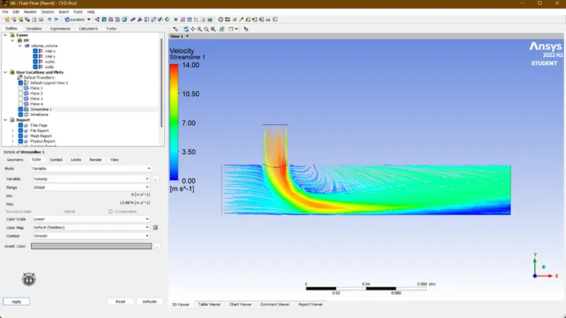
FIG 31. Temperature of long tee (Case 2.1)

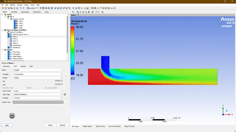
FIG 32. Velocity of long tee (Case 2.1)

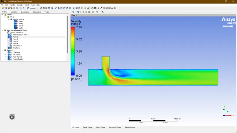
FIG 33. Temperature across the long tee (Case 2.1)

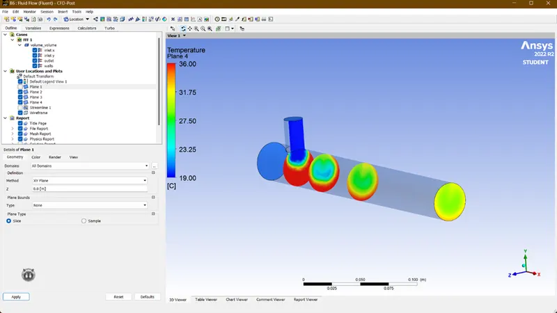
FIG 34. Velocity across the long tee (Case 2.1)

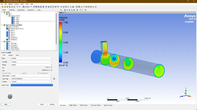
FIG 35. Streamline for Temperature across the long tee (Case 2.1)

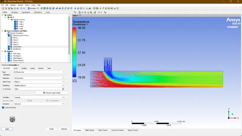
FIG 36. Streamline for Velocity across the long tee (Case 2.1)

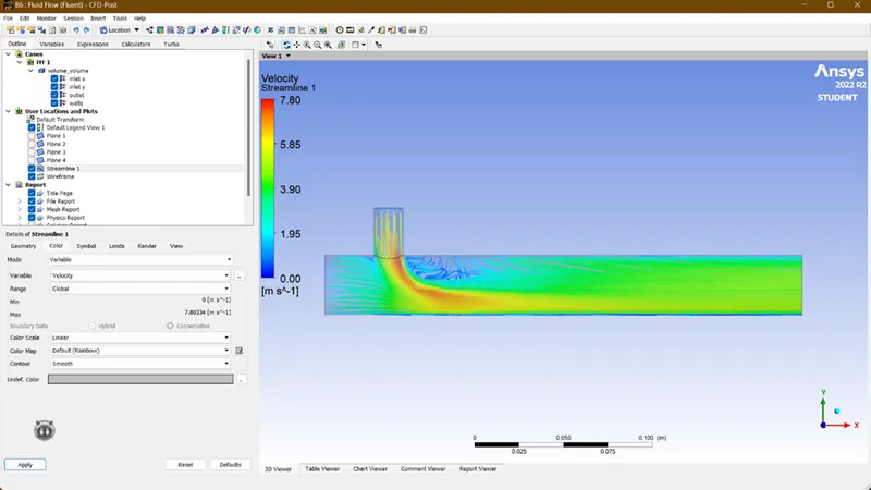
FIG 37. Temperature of long tee (Case 2.2)

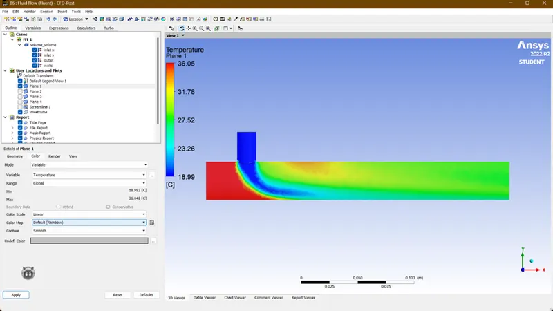
FIG 38. Velocity of long tee (Case 2.2)

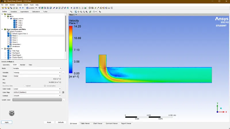
FIG 39. Temperature across the long tee (Case 2.2)

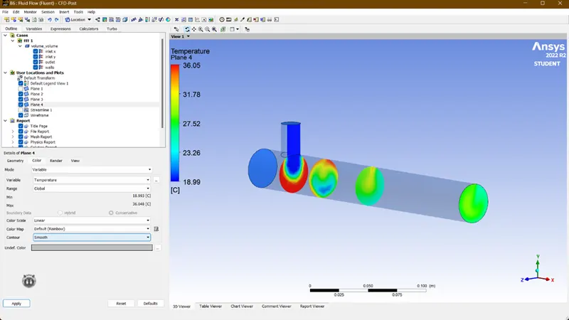
FIG 40. Velocity across the long tee (Case 2.2)

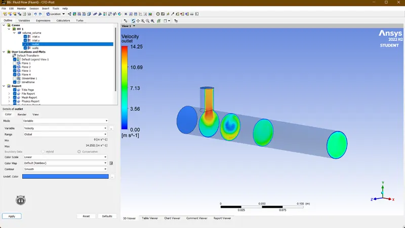
FIG 41. Streamline for Temperature across the long tee (Case 2.2)

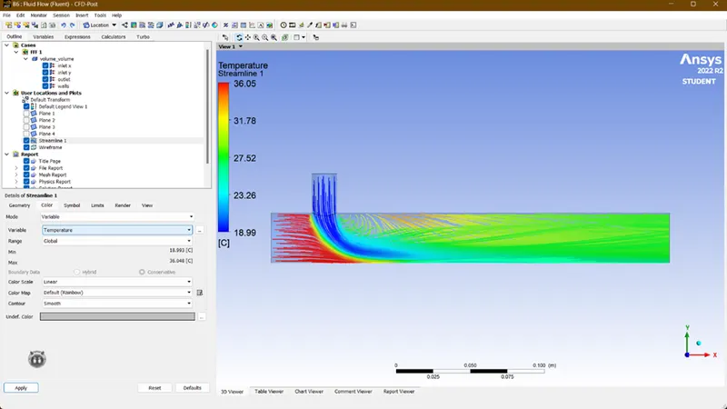
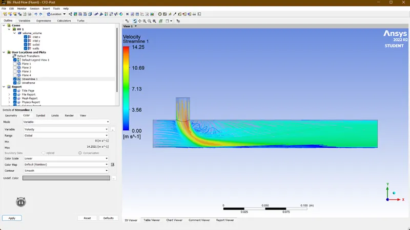
FIG 42. Streamline for Velocity across the long tee (Case 2.2)

GEOMETRY	MOMENTUM RATIO	CELL COUNT	AVERAGE OUTLET TEMPERATURE [C]	NO. OF ITERATIONS TO CONVERGE	NO. OF ITERATIONS	STANDARD DEVIATION
SHORT TEE	2	103737	29	204	250	1.3
SHORT TEE	4	103737	27	300+	300	1
LONG TEE	2	138057	30	161	250	1.1
LONG TEE	4	138057	27	350+	350	0.9

OVERALL DISCUSSION:

AVERAGE OUTLET TEMPERATURE:

Irrespective of length of the mixing Tee, the average outlet temperature on both cases is quite same.

MOMENTUM RATIO:

• As momentum ratio increases, the velocity of cold inlet fluid increases and due to high relative velocity between the fluid it experiences higher turbulence and therefore the outlet fluid temperature decreases.
• For momentum ratio 2, the average outlet fluid temperature is 30C whereas for momentum ratio 4 the average outlet fluid temperature is 27C. From these we can say that there will be a drop in temperature if momentum ratio increases.
• In order to obtain better mixing the velocity of cold air should be increased. By increasing the cold fluid velocity, the outlet temperature gets reduced.

1. OF ITERATIONS:

The longer Tee takes more time to converge than short Tee.

CONCLUSION:

• Higher the momentum ratio, higher will be the mixing efficiency of Tee joint.
• Increasing the length of the pipe does not solve the purpose of mixing efficiently. So, it is efficient to use short pipe.
• The outlet temperature shows significant decrease when momentum ratio is increased resulting in increased mixing efficiency.

Mesh independent study:

• Short Tee model is selected for Mesh independent study.

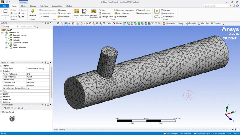
FIG 43. Mesh length of 3mm

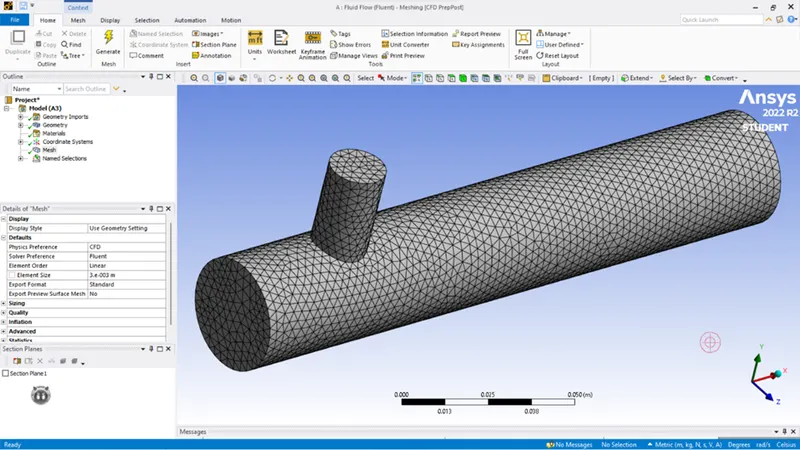
FIG 44. Mesh length of 4mm

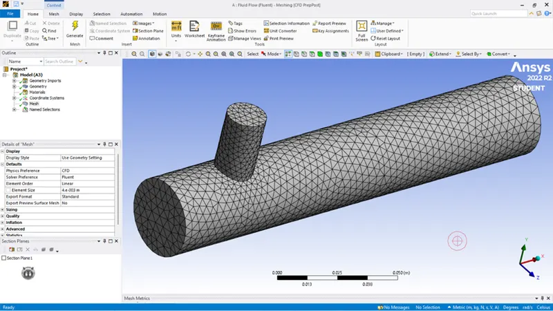
FIG 45. Mesh length of 5mm

RESULTS:

1. 3mm:

FIG 46. Residual plot

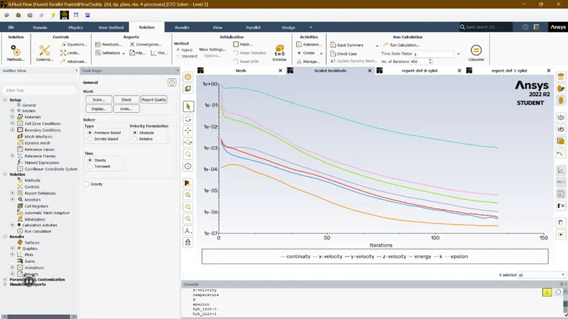
FIG 47. Tavg

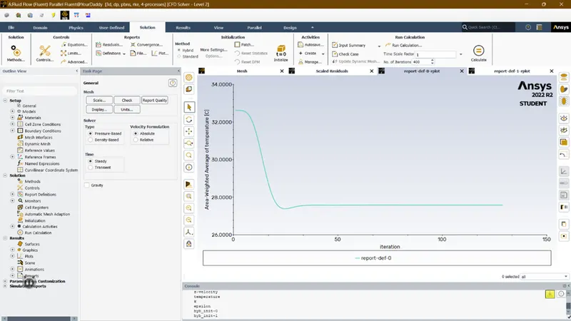
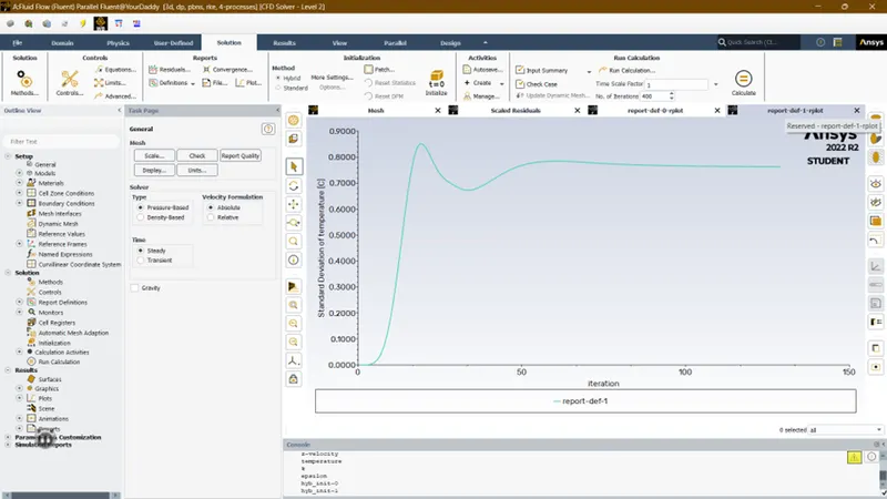
FIG 48. Standard deviation

2. 4mm:

FIG 49. Residual plot

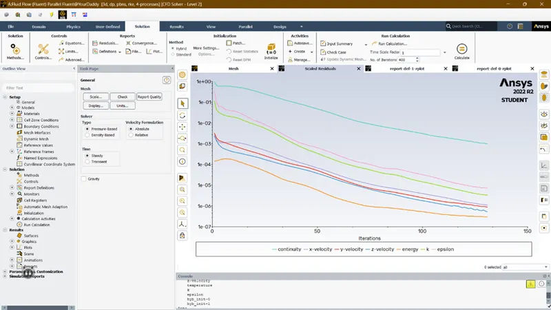
FIG 50. Standard deviation

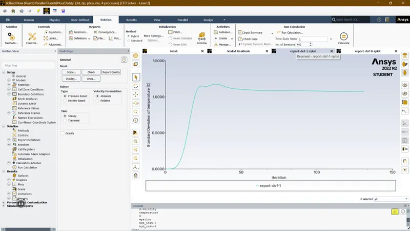
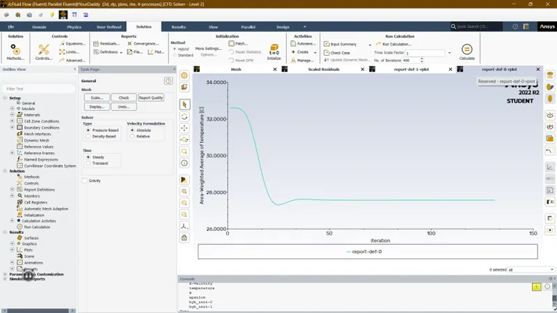
FIG 51. Tavg

3. 5mm:

FIG 52. Residual plot

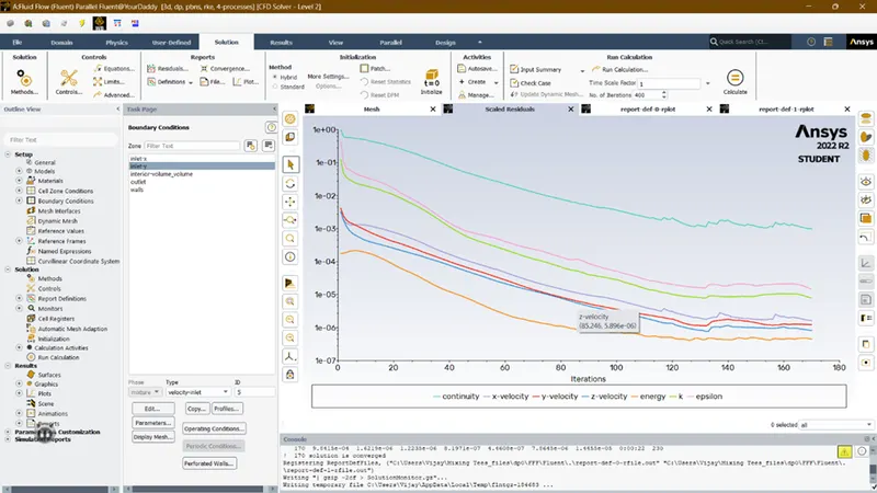
FIG 53. Standard deviation

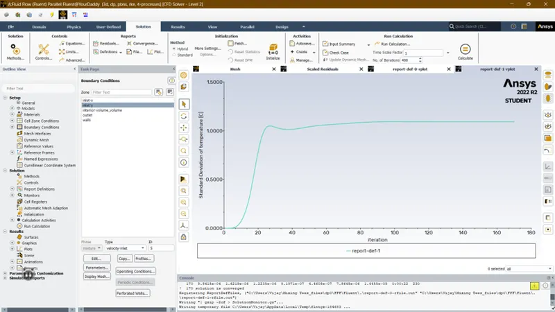
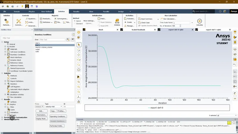
FIG 54. Tavg

CONCLUSION:

• Decreasing the mesh size, the average outlet temperature starts approaching towards the analytical results.