Week 1- Mixing Tee

Aim-

CFD simulation of Tee Mixing with short and long pipe configuration.

Introduction-

CFD is an important tool to create fluid dynamics movies. We can then, with the help of these movies, learn about various parameters of fluid with respect to time and space. Here in this challenge

hot and cold fluids are flowing with their independent flow rates and velocity. The goal of this challenge is to analyze the velocity and temperature plot of these fluids after they directly gets mixed with each other.

Since one fluid is at higher temperature and other is at lower temperature, hot fluid will and cool down releasing heat to the cold fluid which in turn warms it up.

Theory-

This is a classic example of mixed flow. Such type of flow has already been tried in heat exchangers but due to direct mixing and along the flow movement has limited the effecgtiveness of heat transfer.

Here the temperature we get in the outlet completey depends on the mass flow rate and the velocity of the cold fluid i.e. greater the velocity and mass flow rate greater will be the effectiveness of heat tranfer and hence lower will be the temperature at the outlet.

As an evolution out of this later cross and counter flow heat exchangers were invented and now being used widely in the industrial applications. So, one can say that it was one of the stepping stones in the developement of heat exchangers.

The reason I chose k-epsilon model-

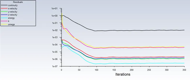
After trying k-epsilon and k-omega model to capture turbulence I found that analysis using k-omega does not converge even after 350 iterations whereas k-epsilon model converges around 130 iterations. So, I chose to go with k-epsilon model for all my further work.

Solving and modelling approach-

1. First I downloaded the models from the information tab in the videos section of the course.

2. Then I started Workbench and created standalone system with ANSYS (Fluent).

3. Double clicked on the Geometry opening the spaceclaim module.

4. Then I imported the respected model in either .stp or .SLDPART extension.

5. Then I extracted the volume that is the space through which fluid flows from Prepare---> Volume extraction---> Selected edge selection and extracted volume by clicking on 'correct' symbol.

6. Then I closed the spaceclaim and double clicked on the mesh.

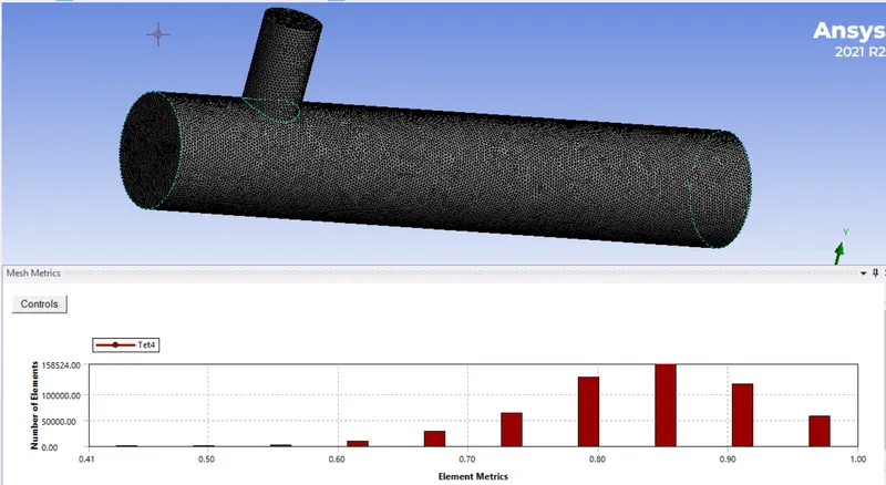
7. In Meshing module, I created named selection at respective faces, then I meshed the model with proper sizing with trail and error method and chose 0.001 m mesh element size.

8. After Meshing I closed Mesh module and double clicked on setup module selected double precision and 6 processors and started Fluent module.

9. In fluent I first checked for material and ensured it was air.

10. Then I chose k-epsilon turbulance model the reason for which I have given in the earlier section.

11. I activeted the Energy equaltion as we are going to study temperature profiles.

12. Then I applied boundary conditions at inlet-x, inlet-y and outlet.

13. In my software the initialization was not converging so I increased initialization iterations to 15 then it got converged.

14. I defined the parameters to study and the location at which they will be studied.

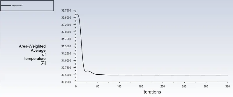
15. I chose area-weighted average for variables and standard deviation to check the error from the actual one.

16. Then I started the calculation for 150 iterations first and it converged at 131 if it had not converged I would have ran the analysis for more iteration untill solution is converged.

Results-

Case 1-

• Short mixing tee with a hot inlet velocity of 3m/s.
• Momentum ratio of 2, 4.

Momentum ratio = velocity at cold inlet / velocity at hot inlet

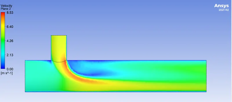
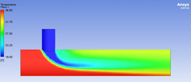
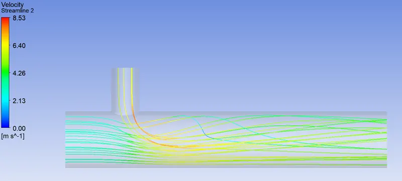
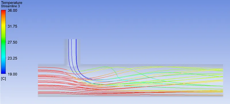
i) Momentum Ratio = 2

Along the length of the pipe=

Velocity Contour Plot- Temperature Contour Plot-

Velocity Line Plot- Temperature Line Plot-

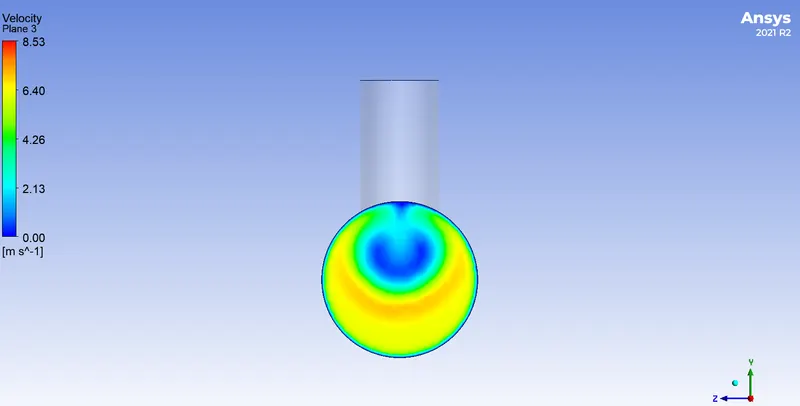
Across the pipe=

Velocity contour plot- Temeprature Contour Plot-

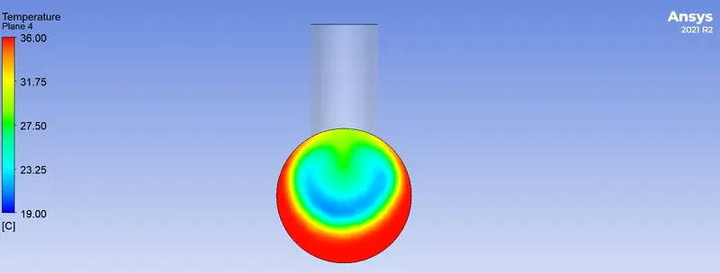
Velocity Line Plot- Temperature Line Plot-

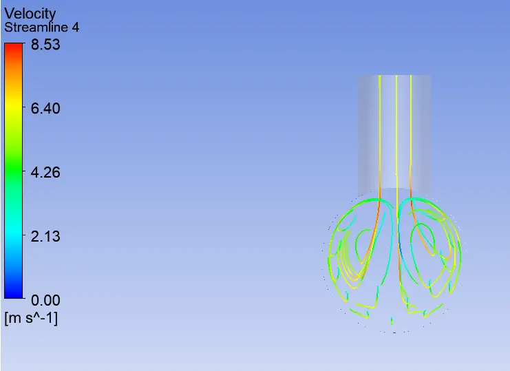
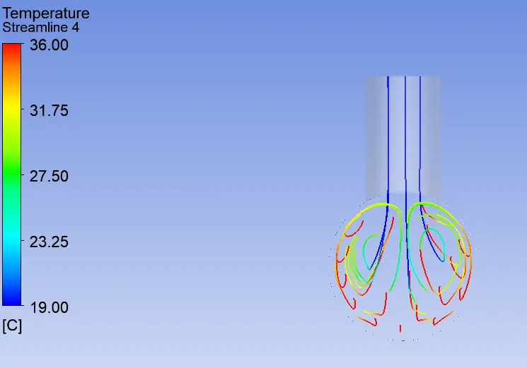
Comparison-

	Momentum Ratio
	Case 1 (Short Tee)		Case 2 (Long Tee)
	2	4	2	4
Cell Count	569312	569312	754654	754654
Average Outlet Temperature	30.562463	27.7089696	30.62764706	27.62975286
Number of Iterations for convergence	131	174	130	262

Conclusion-

1. Momentum ratio has effect on the outlet temperature of the heat exchanger. As momentum ratio increases for the same configuration outlet temperature decreases.

2. For low momentum ratio solution converges within relatively less iterations.

3. As length of the heat exchanger increases outlet temperature decreases as it get more surface area and time for heat transfer. Therefore in long pipe configuration outlet temperature is if not very significantly but sure lower than the short pipe configuration.

4. Longer length takes more interations for solution to converge for momentum ration 4.

5. Since the length is longer element count is also more.