Week 1- Mixing Tee

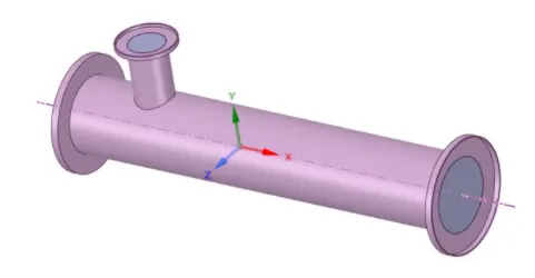
AIM: To set up steady-state simulations to compare the mixing effectiveness when hot inlet temperature is 36⁰C & the Cold inlet is at 19⁰C for different cases described below:

1. Case 1
   • Short mixing tee with a hot inlet velocity of 3m/s.
   • Momentum ratio of 2, 4.
2. Case 2
   • Long mixing tee with a hot inlet velocity of 3m/s.
   • Momentum ratio of 2, 4.

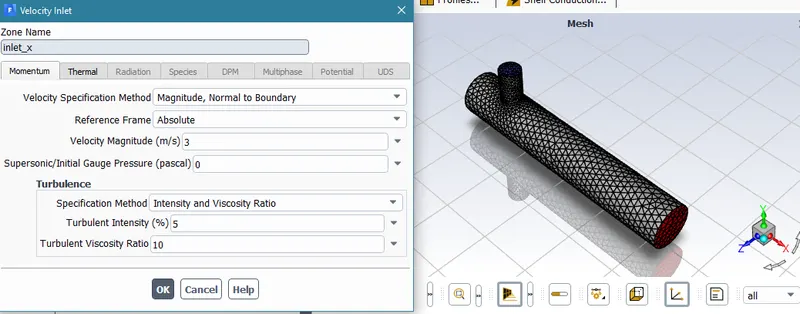
PROCEDURE: CASE 1: The hot inlet velocity is 3 m/s and with a momemtum ratio of 2, the cold inlet velcoity is 6 m/s.

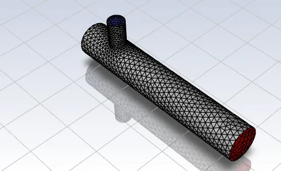
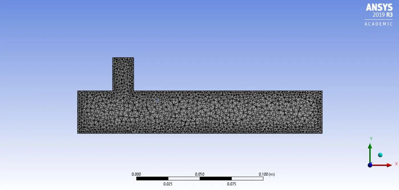
The fluid domain is selected and the preprocessing is done using ANSYS spaceclaim. The meshed model (with total elements as 12657) is shown:

The velocity boundary conditions are setup as shown below: (here for hot inlet)

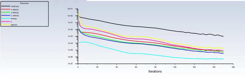
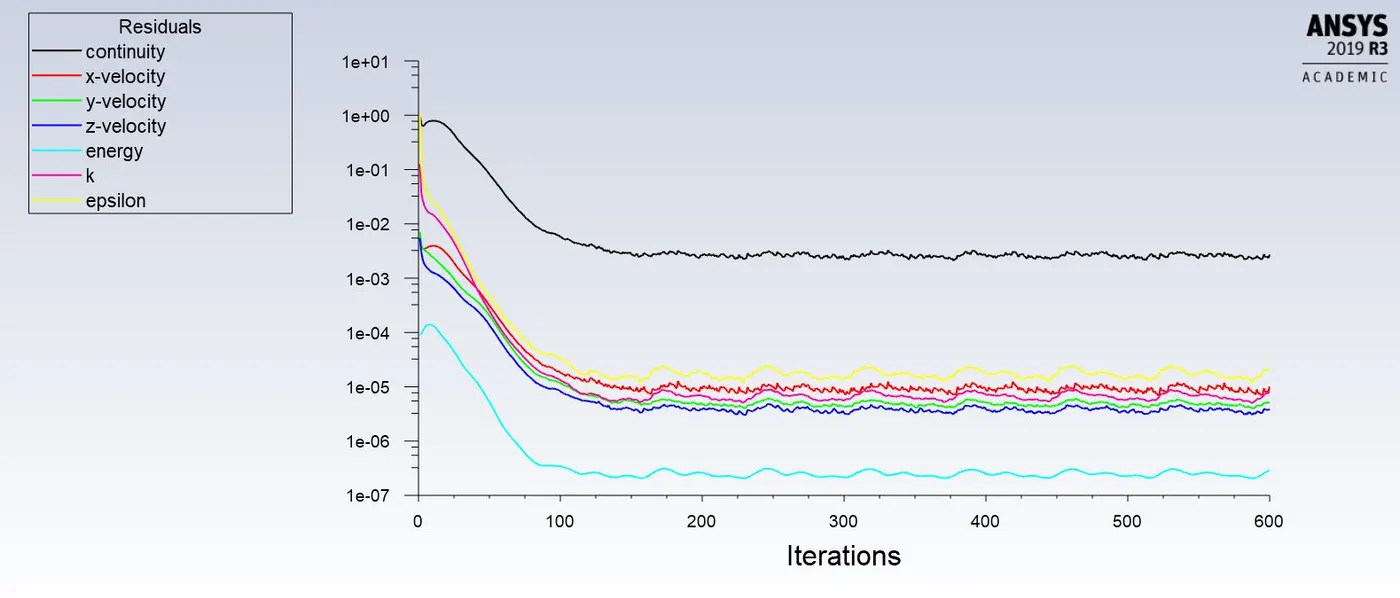
The residual plot for the given case is shown:

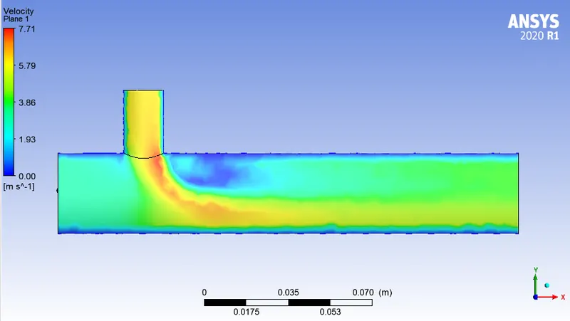
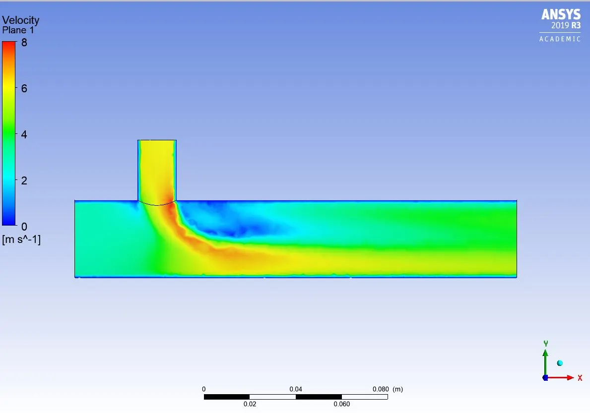
The velocity contours on the cut plane along the length of the pipe is shown:

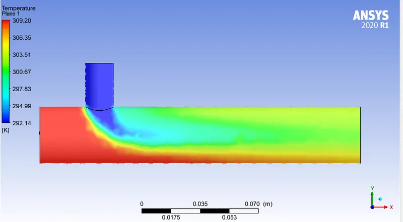
The temperature along the length is shown below:

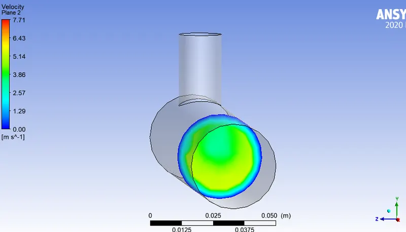
The velocity contour across the length of the pipe at a distance of x=0.05 m from the start of the pipe is shown below:

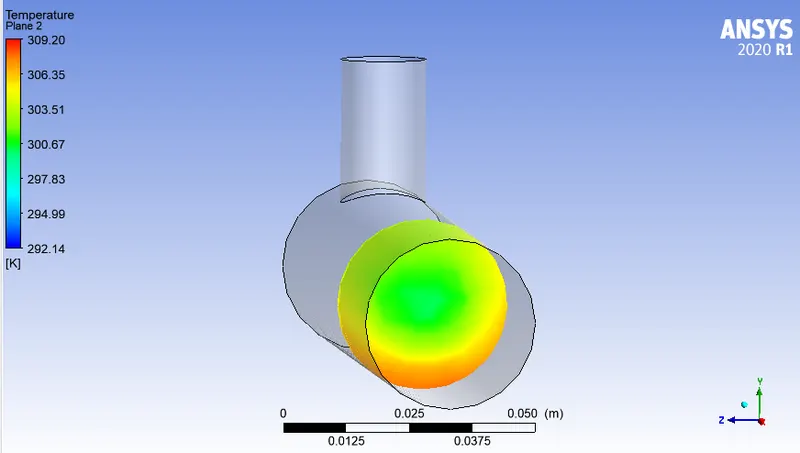
The temperature profile on the same plane is shown below:

For the same case 1, the mesh is now set finer

CASE 1- SHORT TEE, Finer mesh

a) For inlet velocity of 3m/s and momentum ratio of 2

Mesh size- 0.002 m

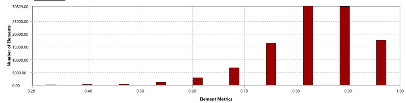
A mesh element metric that identifies the quality of mesh was employed and it can be seen that the elements of the lowest quality are minimal. Most of the elements have quality in the range of 0.7-1. Hence, the mesh is of acceptable quality. The new mesh has total number of elements as 105700.

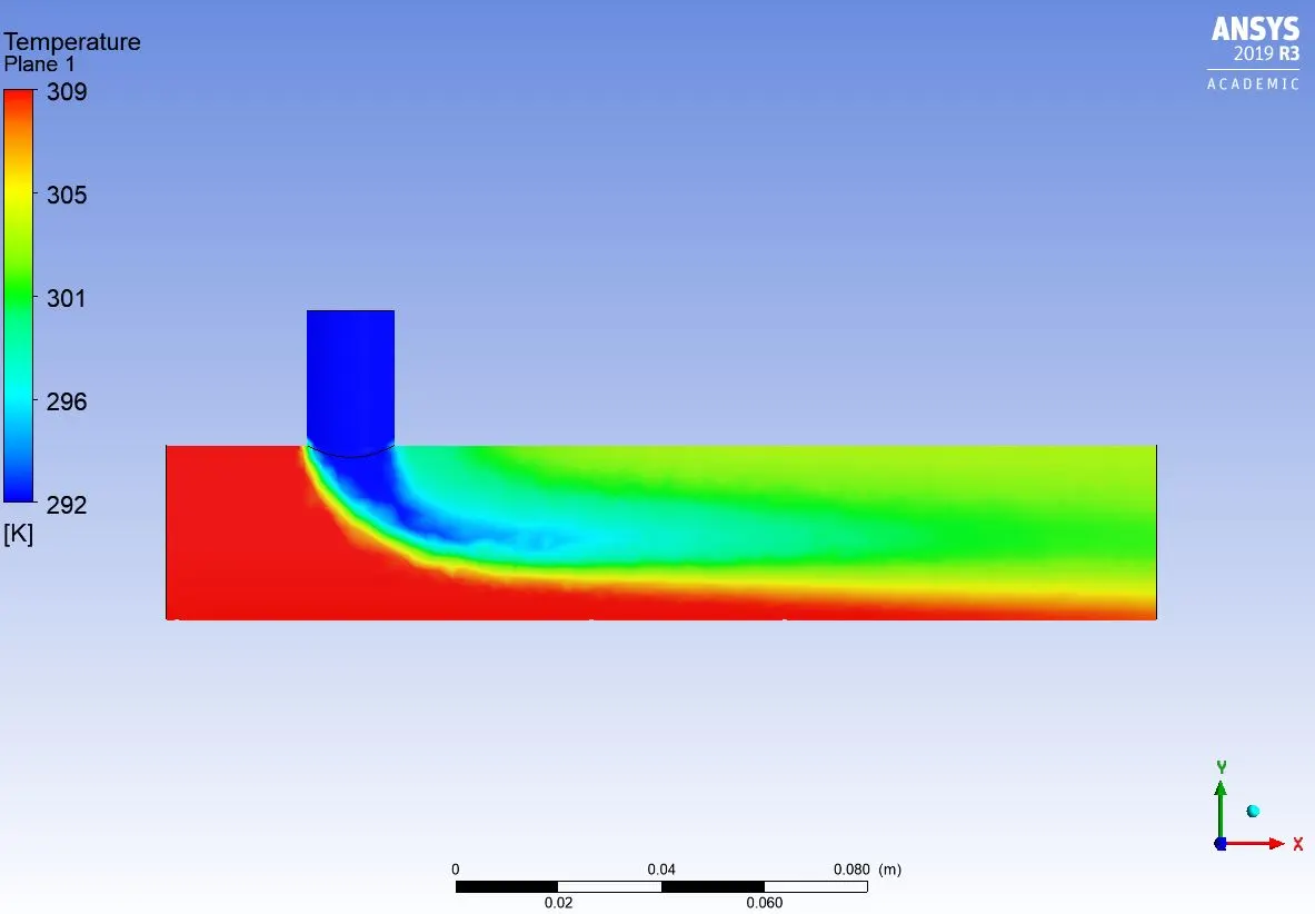
The temperature plot is shown:

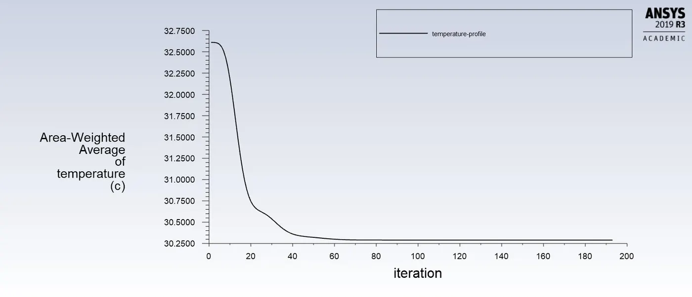
The temperature and velocity plots are shown for the case considered with finer mesh:

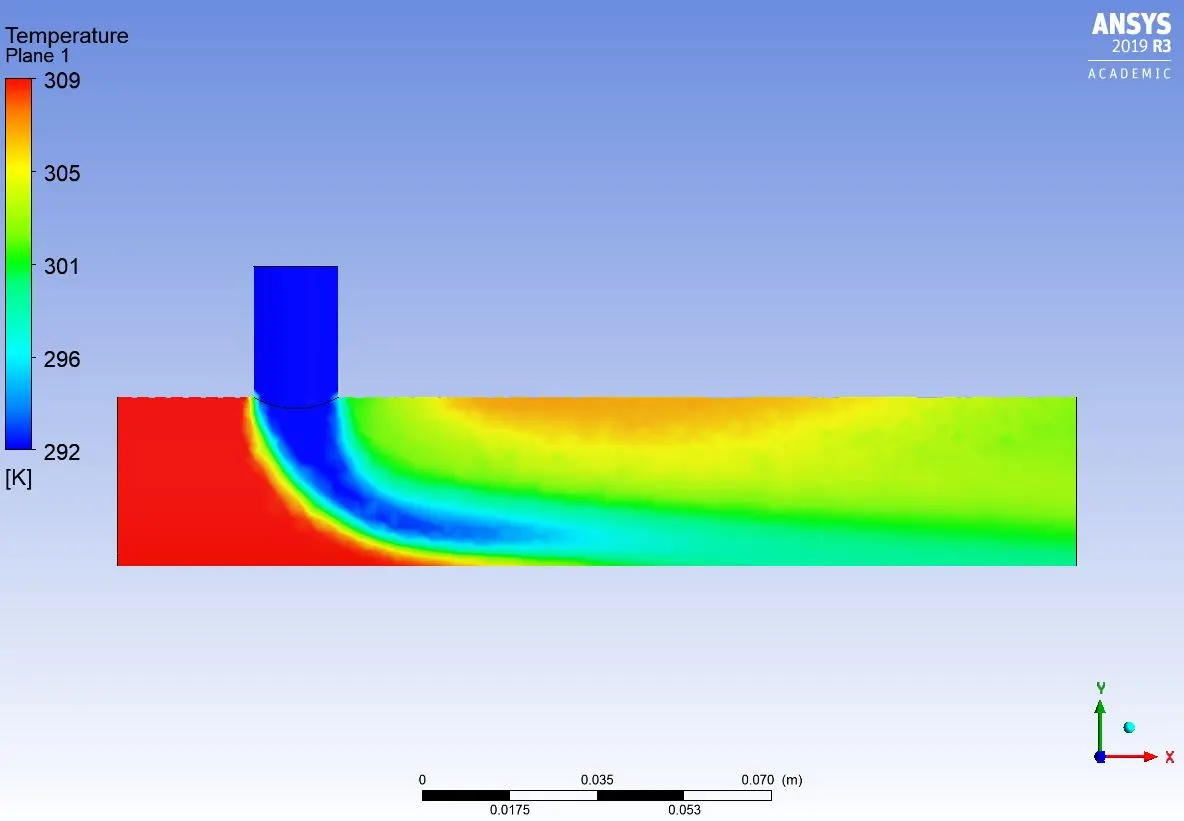
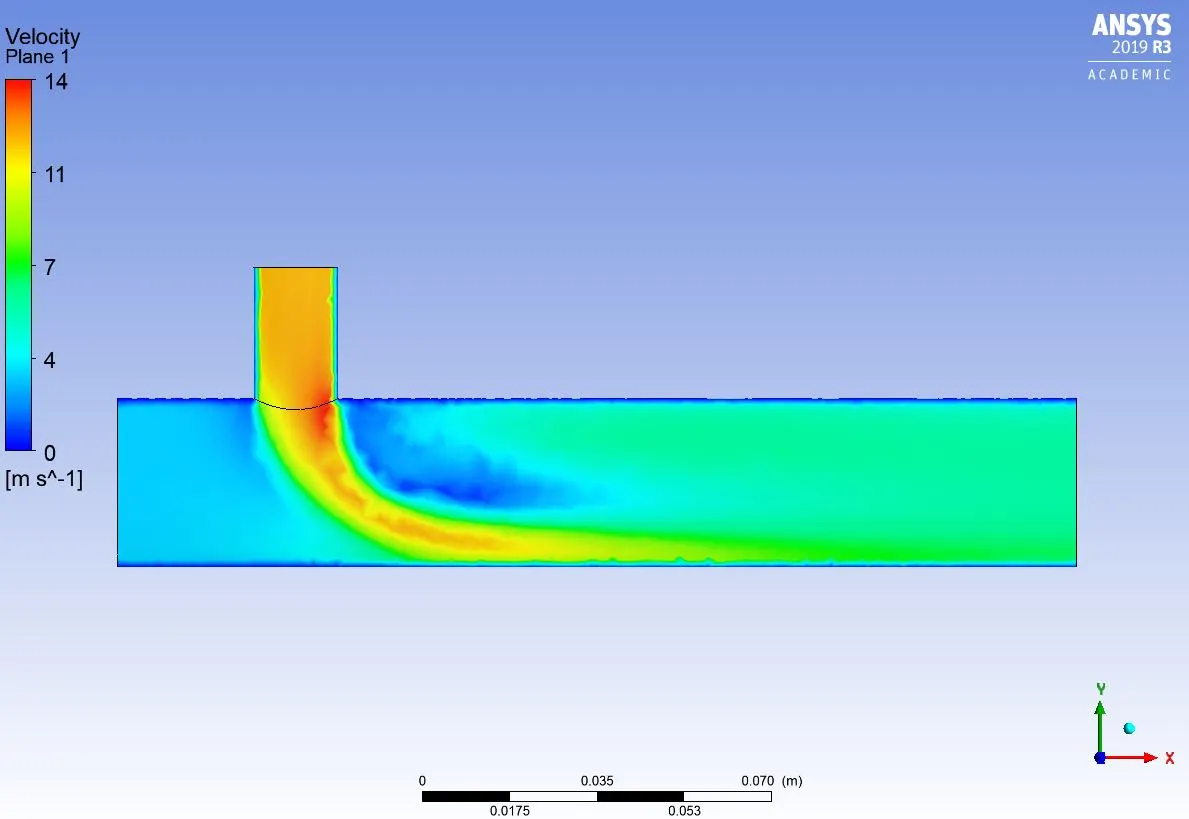
Now with a momemtum ratio of 4, the cold inlet velocity becomes 12m/s. With the same finer mesh as above, the simulated results are shown below:

The temperature and velocity profiles are shown below:

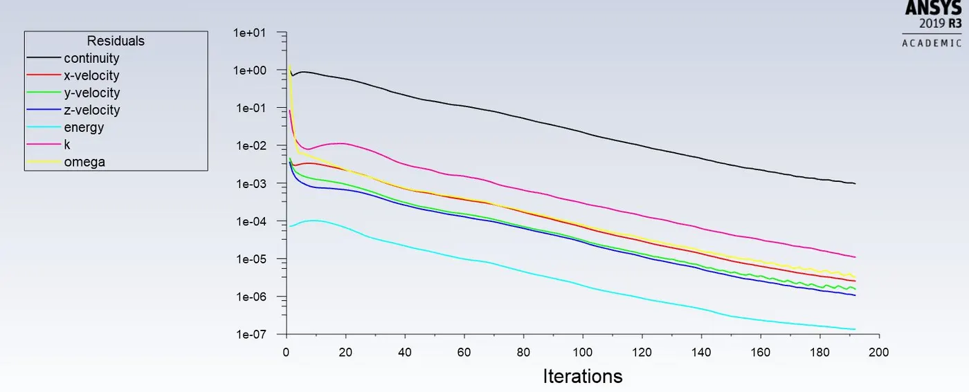
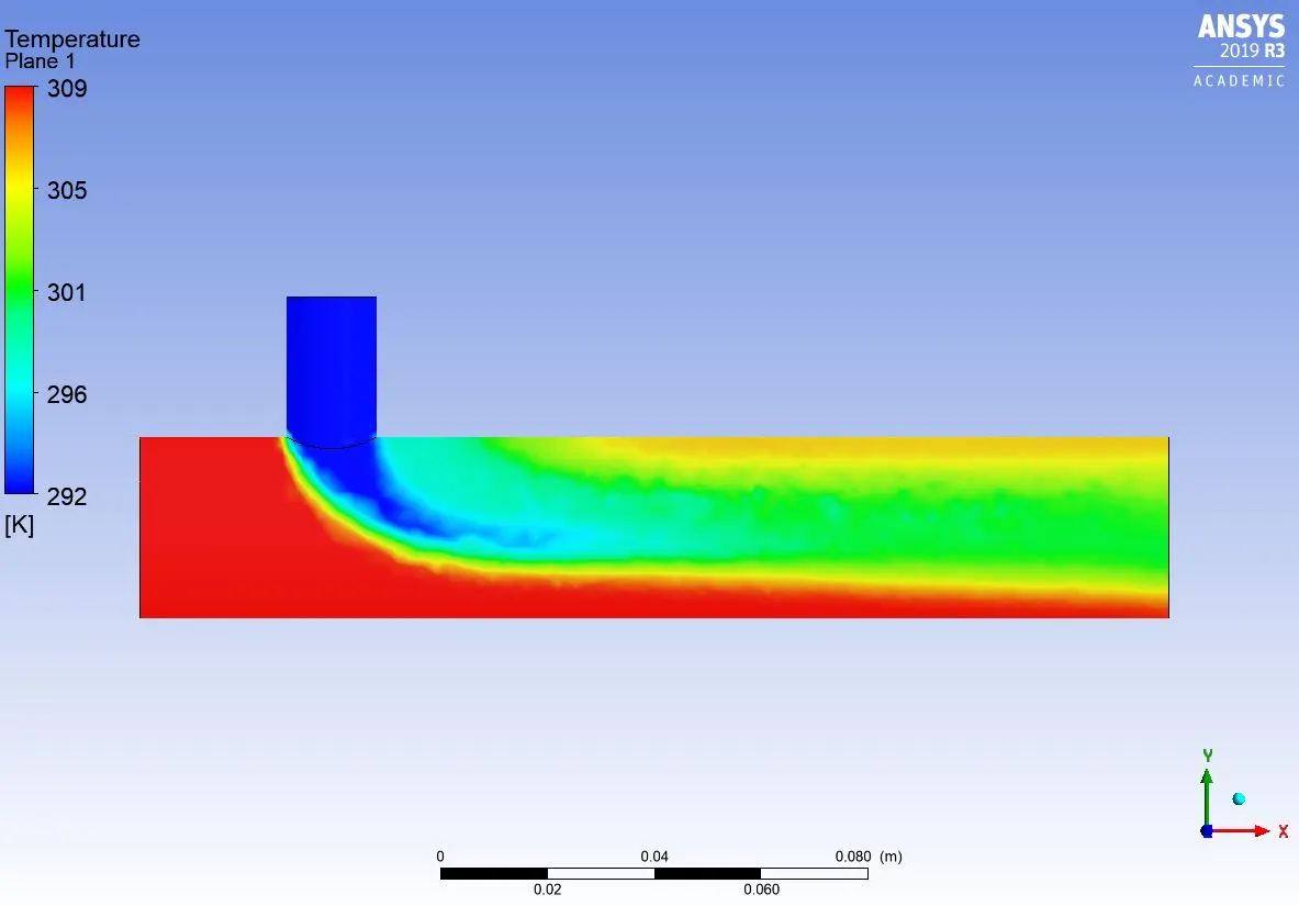
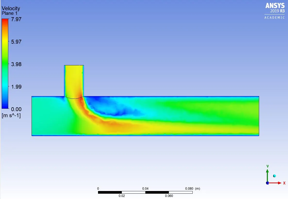
Now, the turbulence model is changed to k-omega and the simulation is run for the short tee with momentum ratio 2, the plots are obtained as below:

The residual plot is shown:

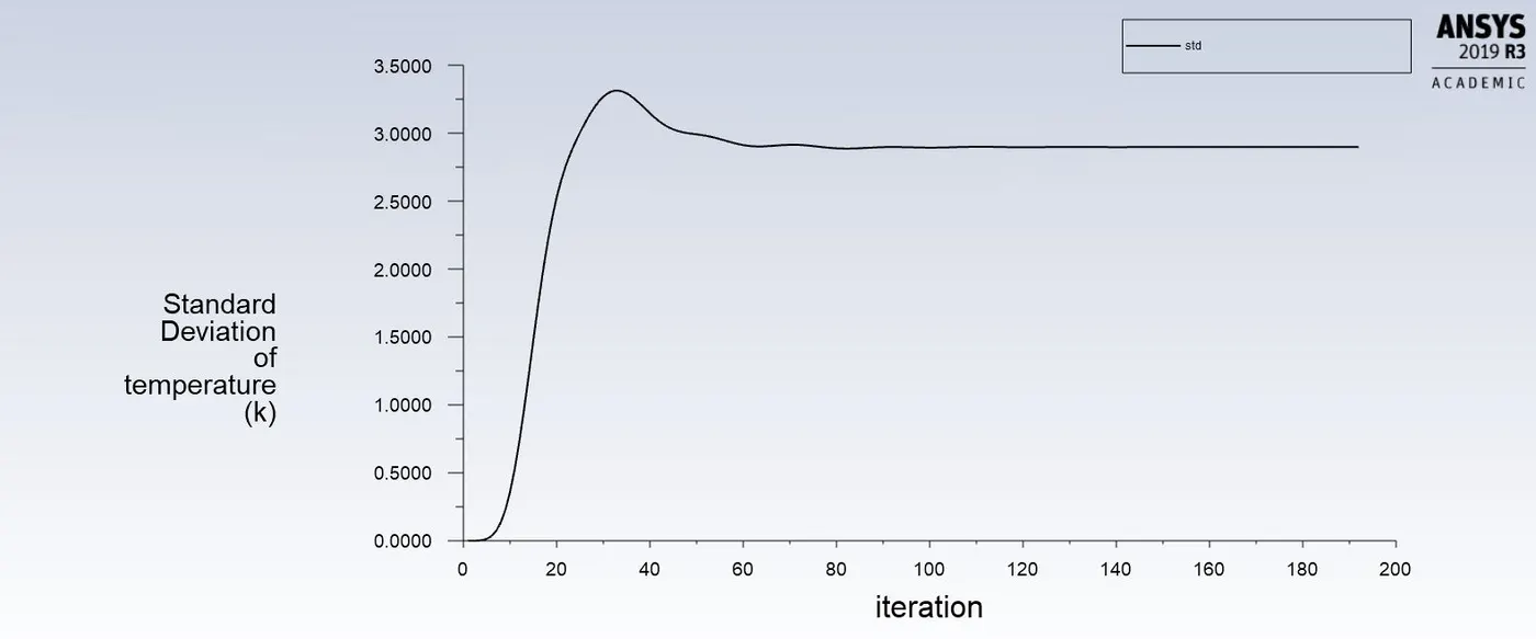
The standard deviation plot is given below:

The temperature and velocity plots are shown:

CASE 2: Simulating for the long tee with same momemtum ratios and comparing the final outlet temperatures:

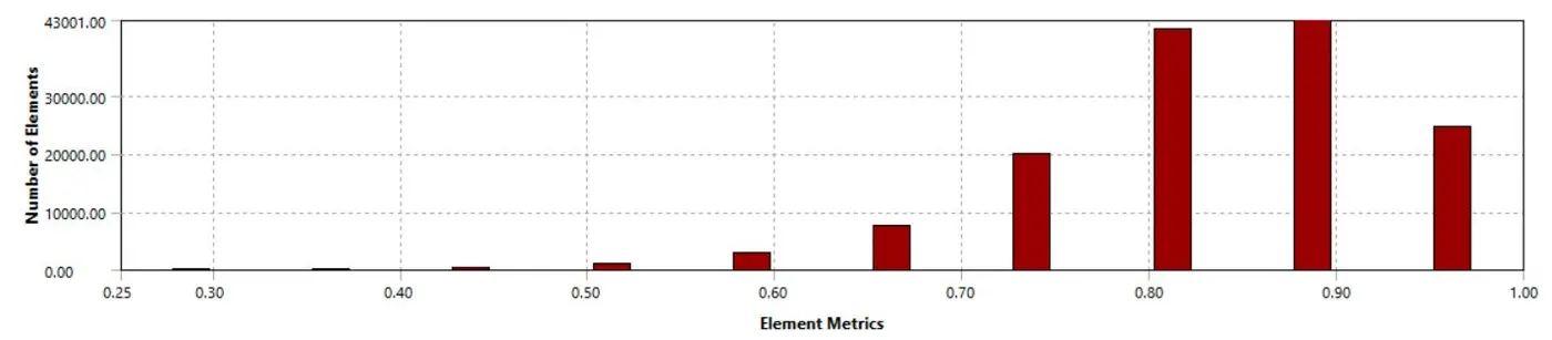
The element metrics graph is shown below. The total number of elements created are now 140500.

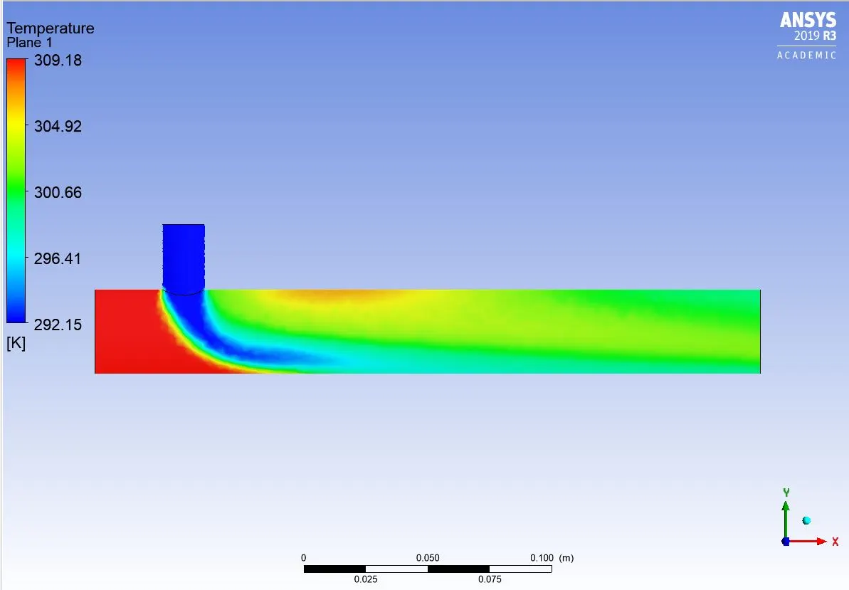
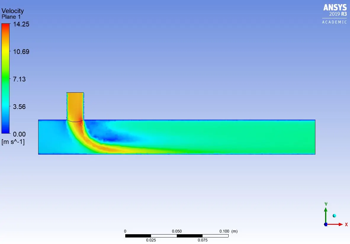
The velocity and temperature contours are shown for a momemtum ratio of 2:

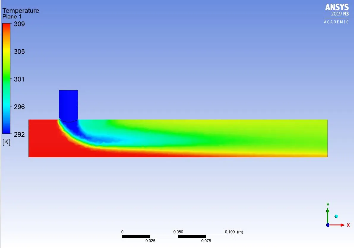
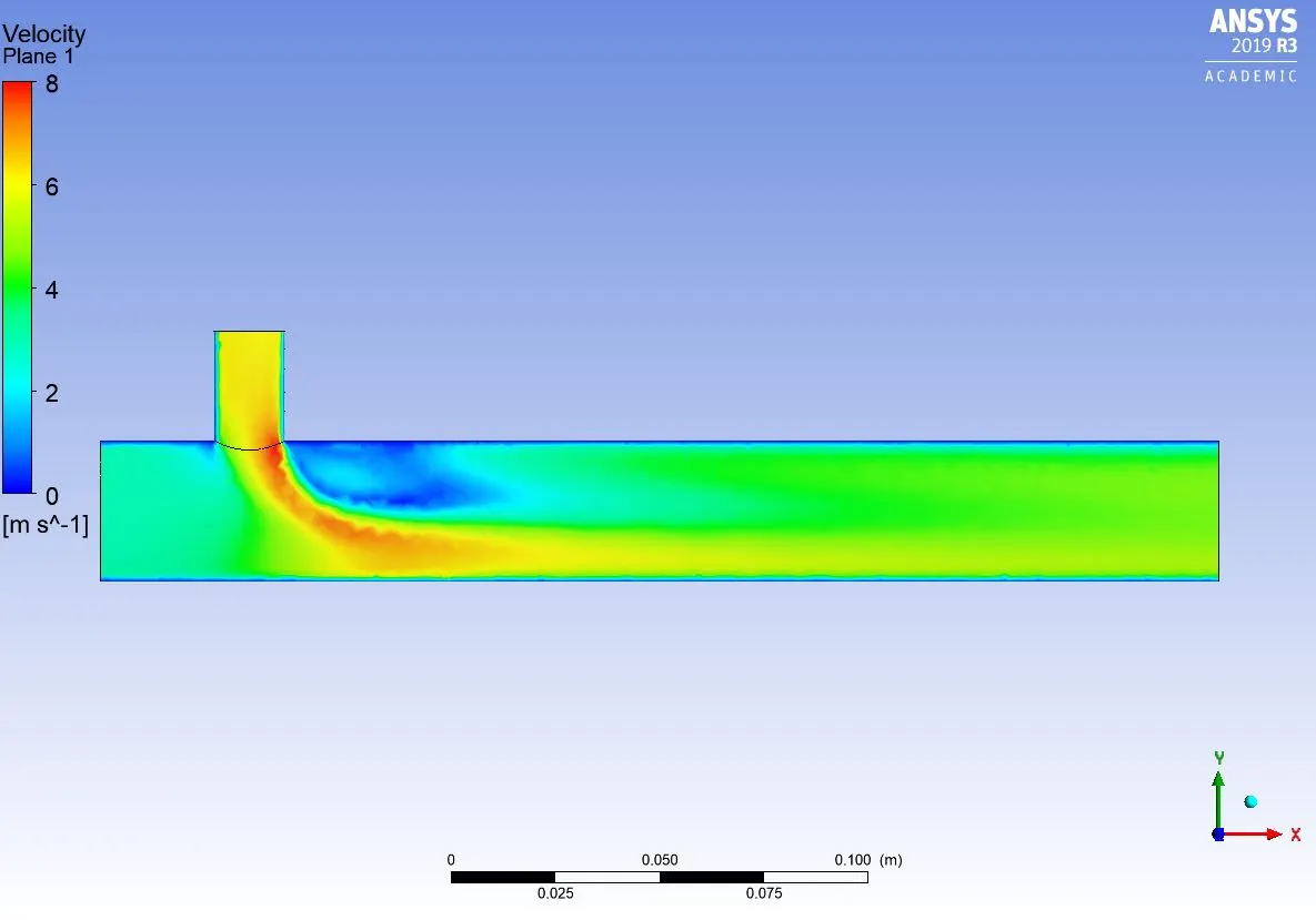
For a momentum ratio of 4, the residual, velocity and temperature plots are shown below:

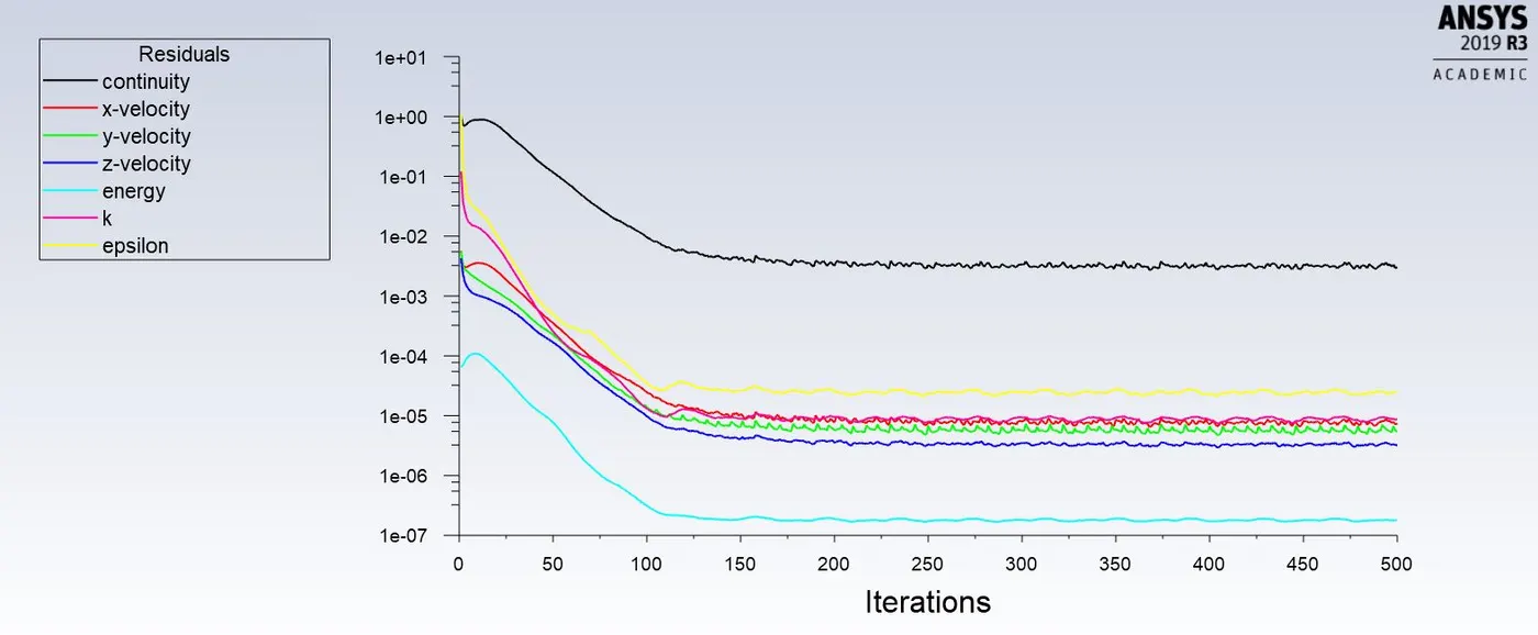
Comparision of results for different cases with finer mesh:

Case	Cell count	Average outlet temperature (K)	Number of iterations for convergence
Case 1, Short tee- Momentum ratio 2	1,05,731	303.45	~ 190
Case 1, Short tee- Momentum ratio 4	1,05,731	300.70	~ 240
Case 2, Long tee- Momentum ratio 2	1,40,500	303.55	~250
Case 2, Long tee- Momentum ratio 4	1,40,500	300.65	~260

Observations:

1) As the momemtum ratio increases, the outlet temperature decreases significantly due to high velocity of cold air from the inlet and increased turbulent mixing.

2) As the length of the tee increases, there is a proper mixing of high temperature flow along the length with the cold air temperatures. hence the outlet temperatures are relatively lower than that of short tees.

3) A long tee with higher momentum ratio will result in the lowest outlet temperature.

3) k- epsilon model predicts well far from the boundaries (wall) and k- omega model predicts well near the wall. Since the current problem focuses more on the outlet temperatures and not at the walls, the k -epsilon model is chosen for all the simulations.