Week 1- Mixing Tee

Objective:

Setup a steady state simulation to determine and compare a average outlet temperature and mixing efficiency of a fluid for two different Tee Pipe with different Momentum Ratio's using Ansys Fluent

Introduction:

piping systems occurs in the various applications do not always have a straight pipe geometry. The configurations of these pipelines are usually zigzag or snake-like in order to provide a good layout flexibility in the limited space. Therefore, the pipe fittings and joints, such as elbows, blind tees, T-junctions and Y-junctions, are commonly adopted in these piping systems. A Tee joint is used to connect two different or same diameter pipes at an angle 90 degrees.Tees may also be used for mixing a two different liquids or same liquid with different properties.Tees with same diameter is said to be equal Tee(Branch size= Run size),with different diameter is said to be reducing tee (Branch size < Run size).Tee Joints are manufactured based on various standards like ASTM A403(Wrought austentic Stainless Steel Piping Fittings),ASTM A 234(wrought carbon steel and alloy steel fittings of seamless and welded construction),ASME B16.9(Factory-Made wrought Steel Buttwelding Fittings),MSS SP-43(Wrought and Fabricated Butt welding fittings for low pressure,corrosion resistant applications),DIN 2615(steel Butt welding pipe fittings),DIN 2616(steel Butt welding pipe fittings) ,NF EN10253-1(wrought carbon steel butt welding pipe fittings),BS EN10253-2 (Non alloy and ferritic alloy steel butt welding pipe fittings) etc..,.The fluid flow at the connections or joint parts of the pipelines behaves differently from the flow of fluid in a straight pipe as reported by Humphrey et al. (1985), Soleimani (1999) and Vasava (2007).probably,investigation of the flow behaviour and flow properties becames significant at the Joints and fittings.A Tee pipe choosen for study is also similar to the Tee Joint

some of the formulas required to carry out simulations are

momentum ratio=`frac{underset(hot)(V)}{underset(cold)(V)}`

`underset(hot)(V)=`velocity of hot inlet in x-direction (`frac{m}{s}`)

`underset(cold)(V)=`Velocity of cold inlet in y-direction (`frac{m}{s}`)

Average of final temperature of two mixtures given by

`underset(mixture)(T)=frac{underset(hot)(m)*underset(hot)(T)+underset(cold)(m)*underset(cold)(T)}{underset(hot)(m)+underset(cold)(m)}`

`underset(hot)(m)=`mass of hot fluid

`underset(cold)(m)=`mass of cold fluid

`underset(cold)(T)=`Temperature of cold fluid (in celcius)

`underset(hot)(T)=`Temperature of hot fluid (in celcius)

Procedure:

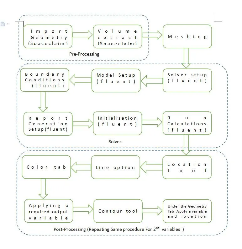
1.Procedure would be followed for the multiple cases from short tee case chart.

2.procedure would be followed running a simulation with long tee pipe for two momentum ratios

Pre-processing:

Geometry:

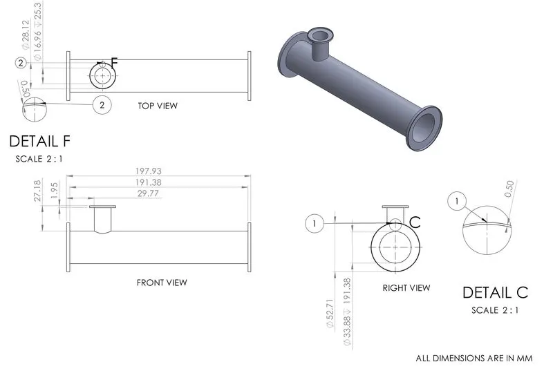
1.Short Tee Pipe

2.Long Tee Pipe

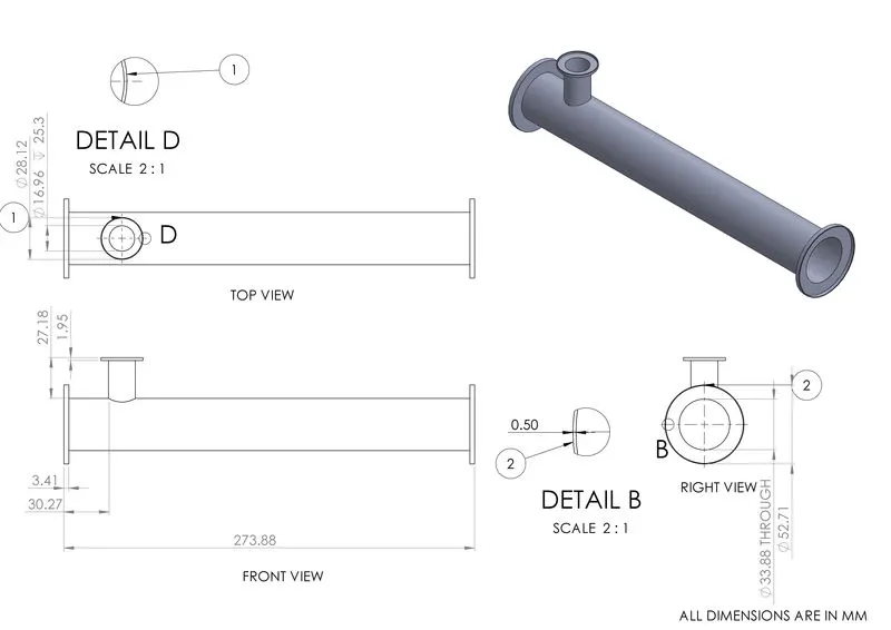
Each Geometry is used to Extract a volume.

Difference between the Geometry is the length of 100 mm

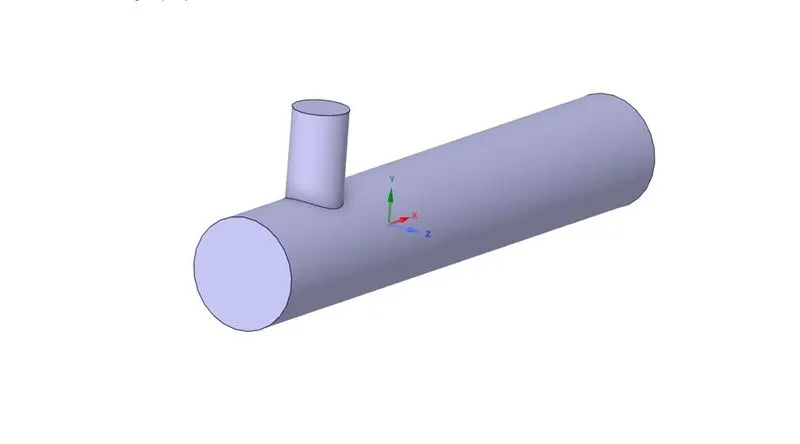
Volume Extract

Short Tee and long Tee looks similar to given below

SOLVER:

Solver Setup:

A steady state solver is choosen to study

the flow behaviour in steady state.

Pressure based solver is used to study about incompressible flows.

viscous Model Setup:

inviscid is not suitable for flow in a pipe.

Laminar model is not suitable for the turbulent flow.

spalarat - Allmaras is not suitable for free shear flows and it is not calibrated to industrial applications.

`K-epsilon`is a turbulence model calibrated for the industrial applications.

`K-omega` is also a turbulence model suitable for low reynolds number regions.

Beyond these model will have a more than two transport equation will leads increase the computational cost per iteration

`K-epsilon` model

1.Standard - Performs poorly for flows with larger pressure gradient, strong separation, high swirling component and large streamline curvature,Inaccurate prediction of the spreading rate of round jets.Production of k is excessive (unphysical) in regions with large strain rate (for example, near a stagnation point), resulting in very inaccurate model predictions

2.RNG -Performs better than standard model for more complex shear flows, and flows with high strain rates, swirl, and separation

3.Realizable-Accurately predicts the spreading rate of both planar and round jets,superior performance compared with the standard k-epsilon model for flows involving rotation, boundary layers under strong adverse pressure gradients, separation, and recirculation

selecting the `K-epsilon`Realizable model to avoid the poor performation of pressure gradients.

`K-omega` model

1.Standard-Well suited for simulating the flow near the wall.

2.Shear Stress Transport (SST)- blended function gradually transition from the standard `K-omega` model near the wall to a high-Reynolds-number version of the `k-epsilon` model in the outer portion of the boundary layer

Selecting the `K-omega` SST model to avoid poor estimation at outer portion of boundary layer.

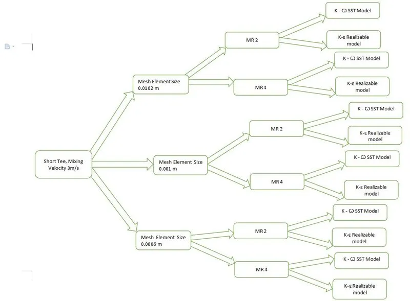
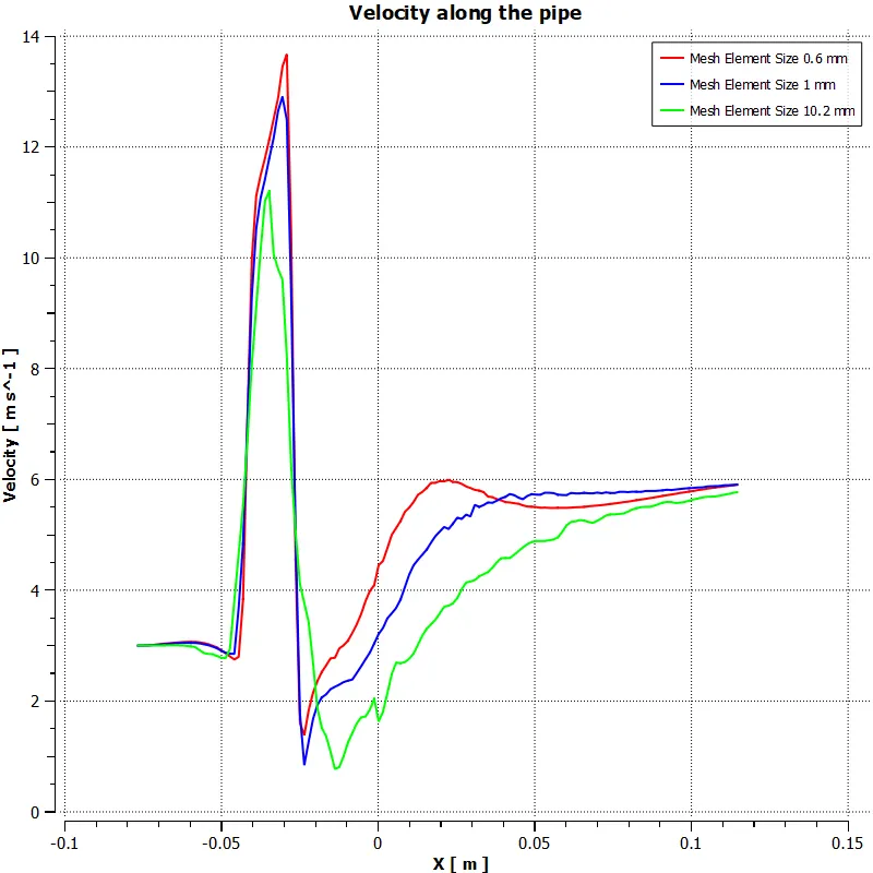
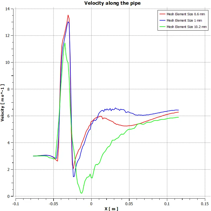
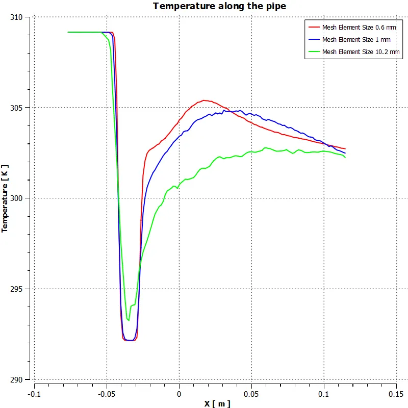
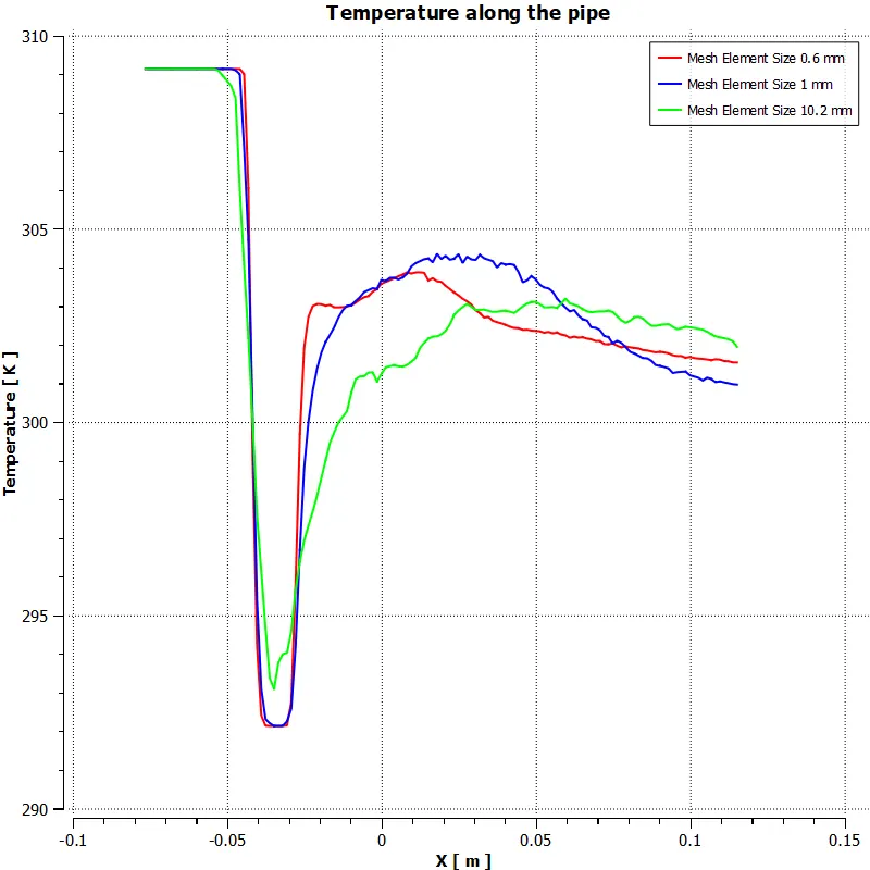
Short tee cases chart (viscous model and mesh independent)

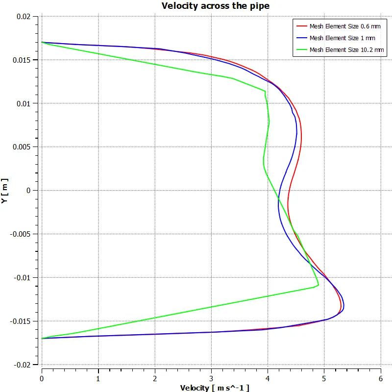
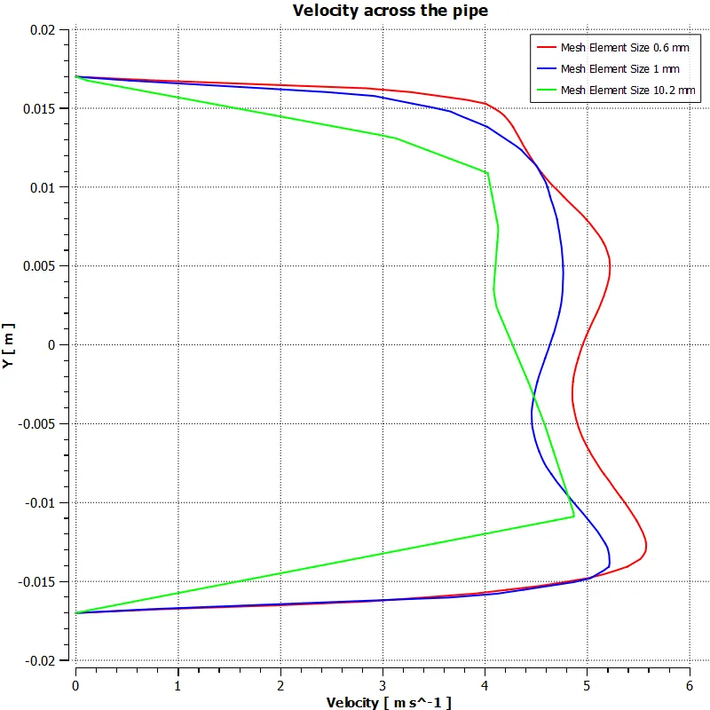
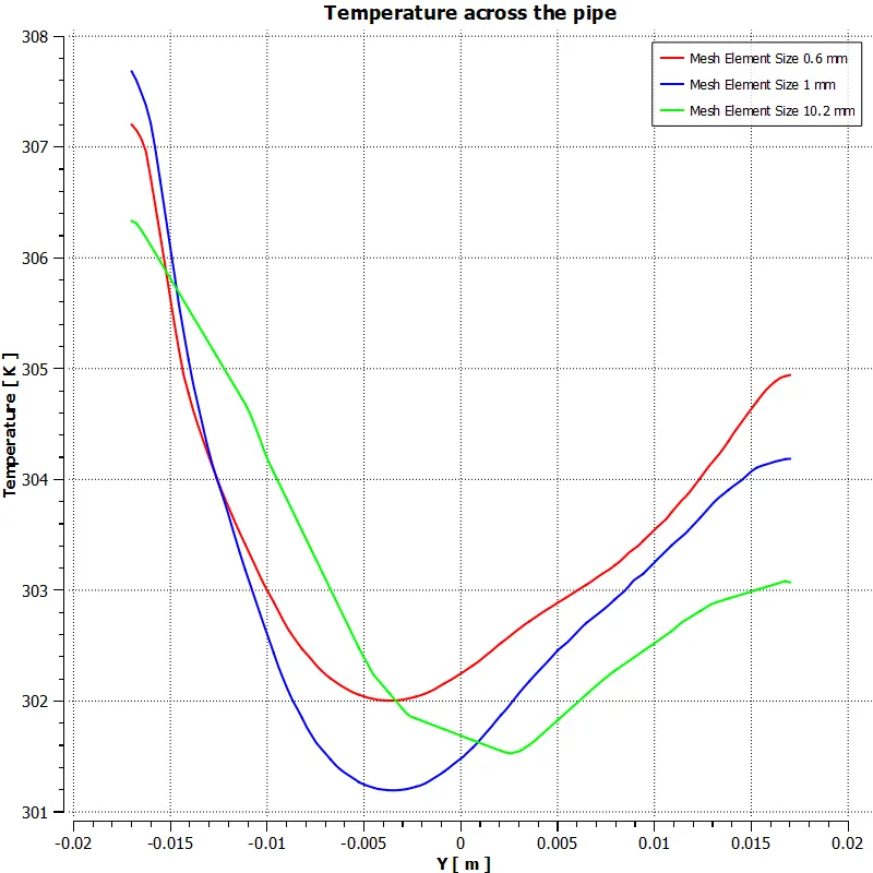
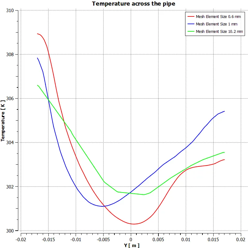
Plot:

`K-epsilon` Realisable Model	`K-omega` SST Model
Momentum Ratio 2	Momentum Ratio 2
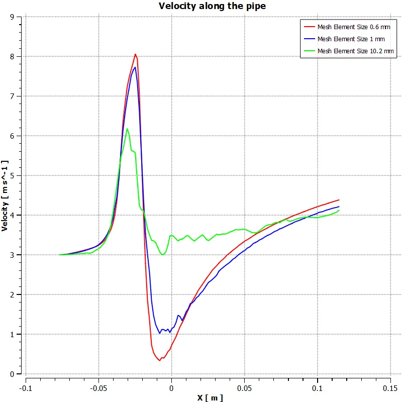
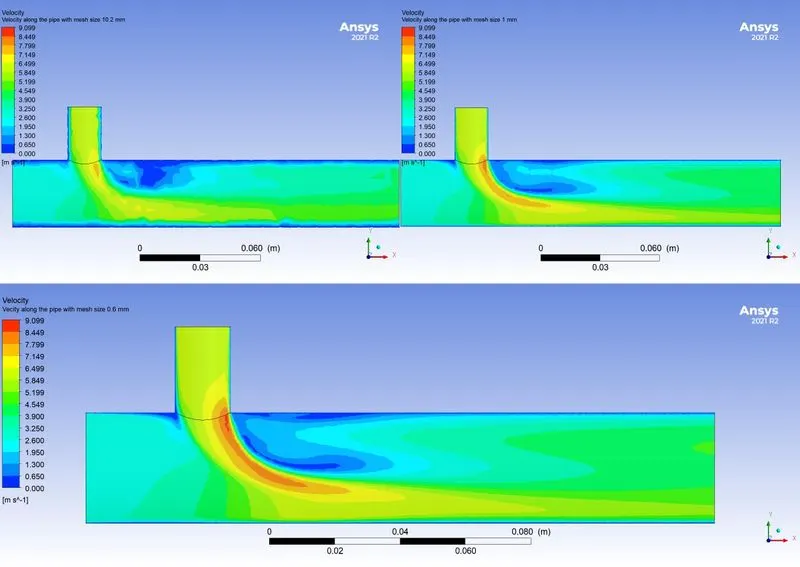
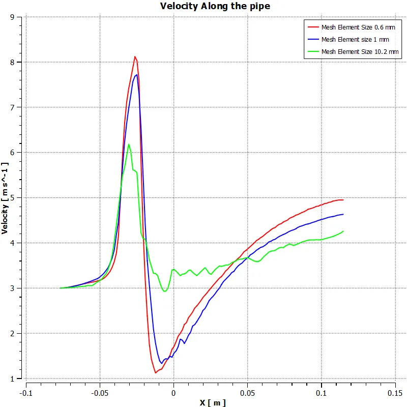
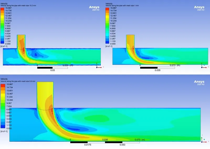
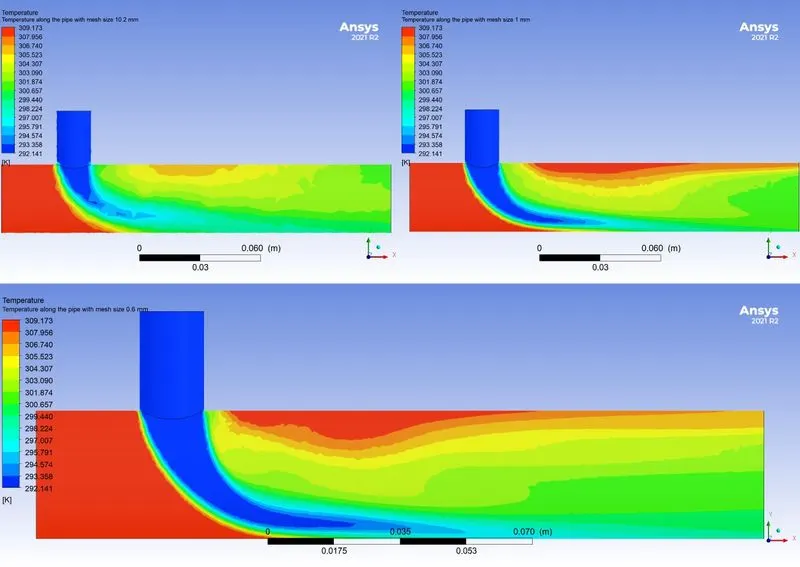
Comparision of velocity along the pipe for three different mesh element size.	Comparision of velocity along the pipe for three different mesh element size.
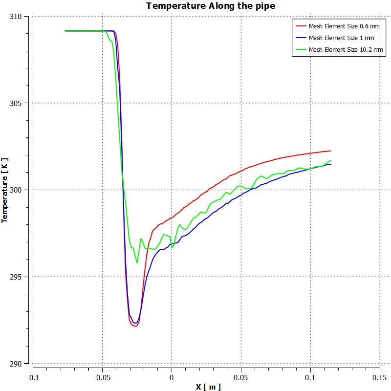
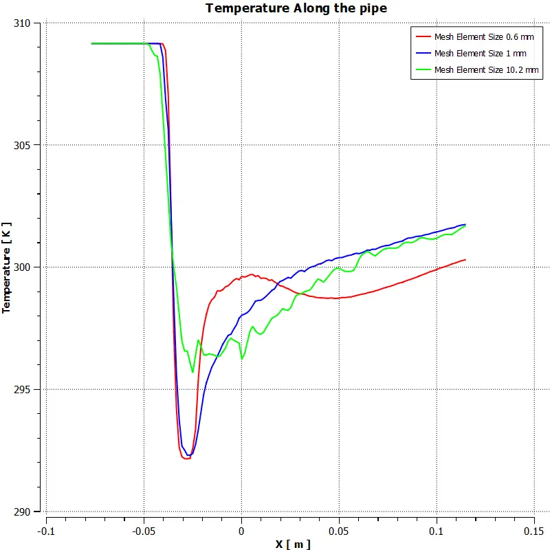
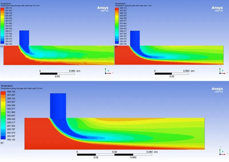
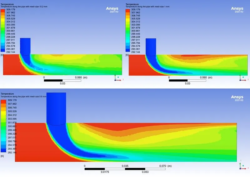
Comparision of temperature along the pipe for three different mesh element size.	Comparision of temperature along the pipe for three different mesh element size.
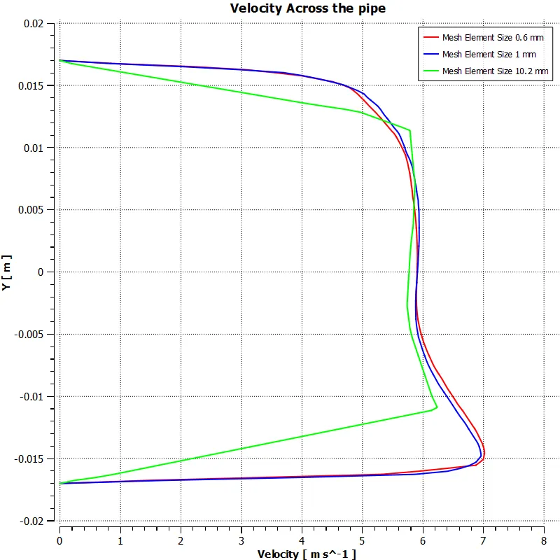
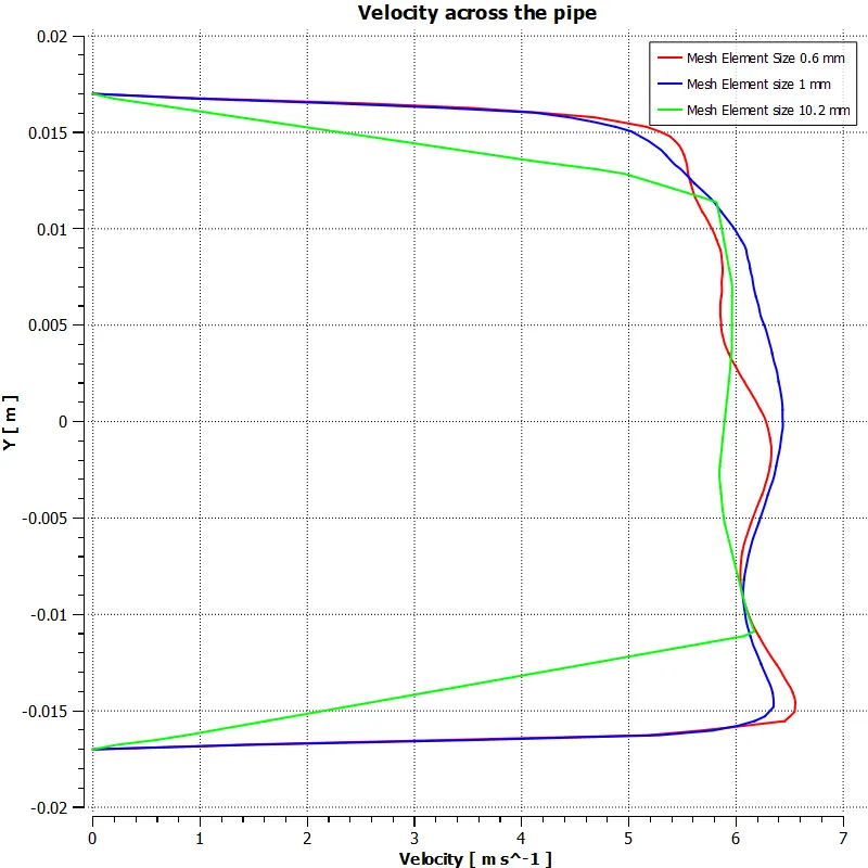
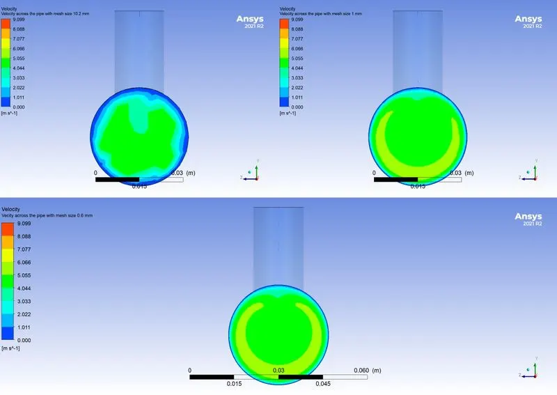
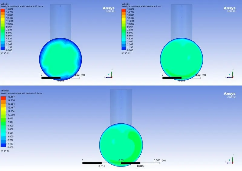
Comparision of velocity across the pipe for three different mesh element size.	Comparision of velocity across the pipe for three different mesh element size.
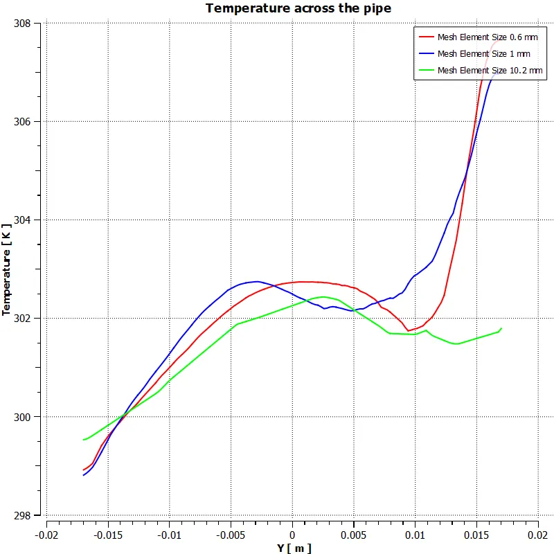
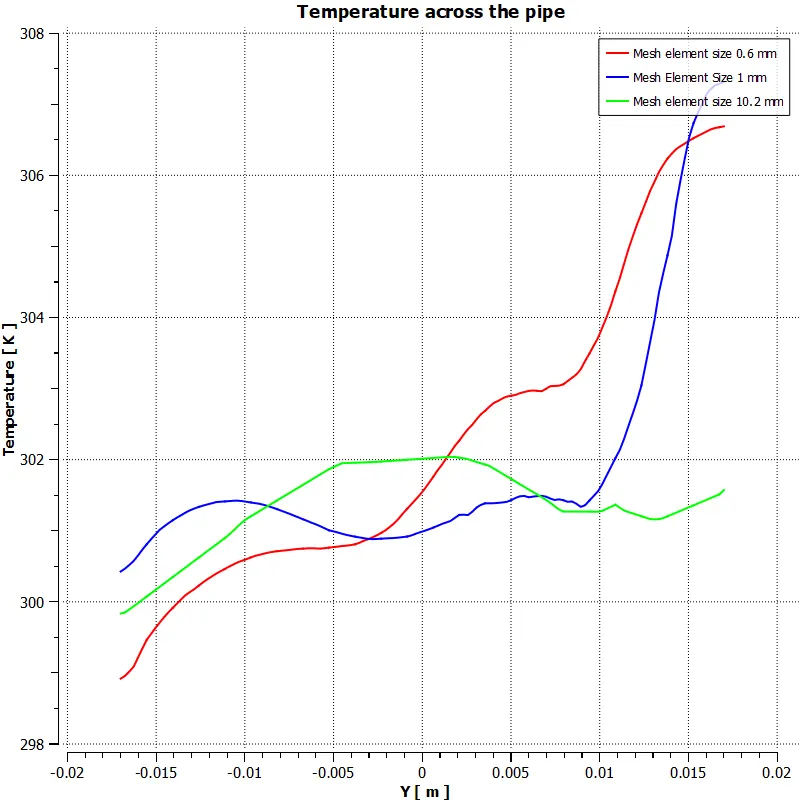
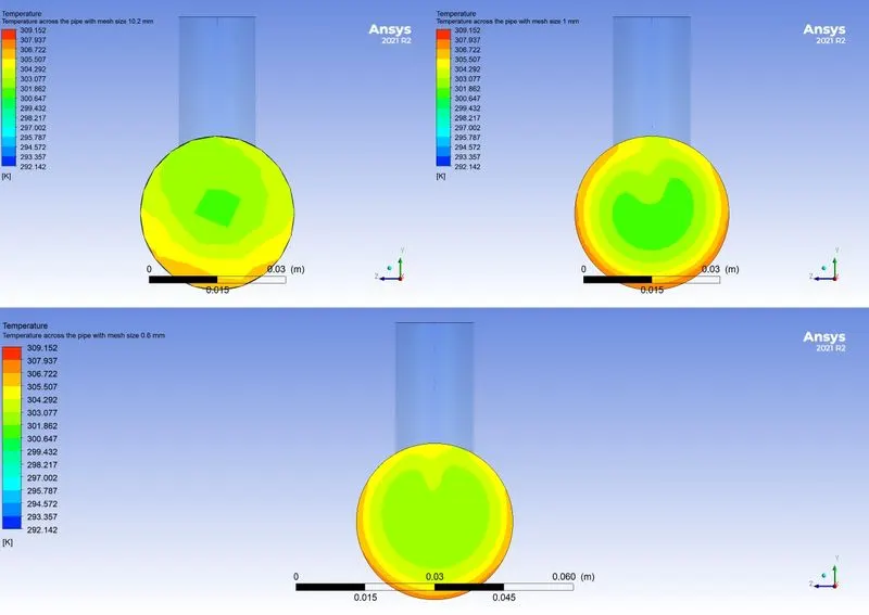
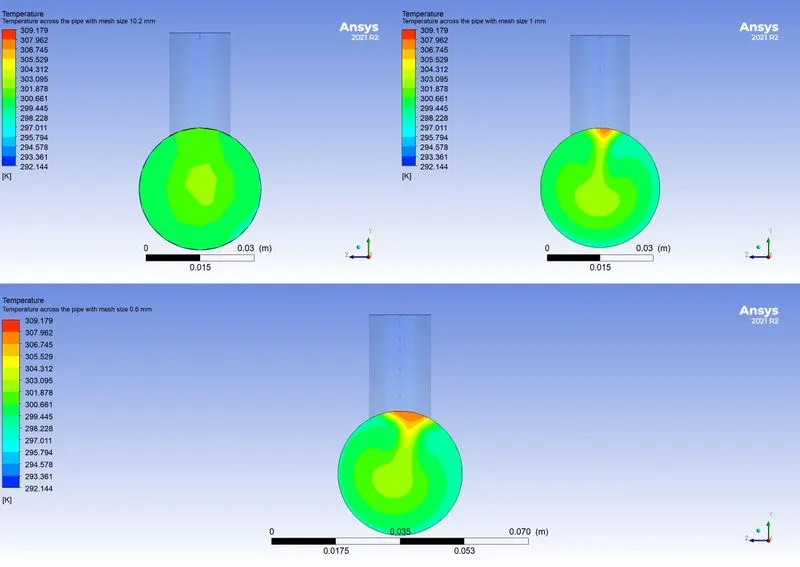
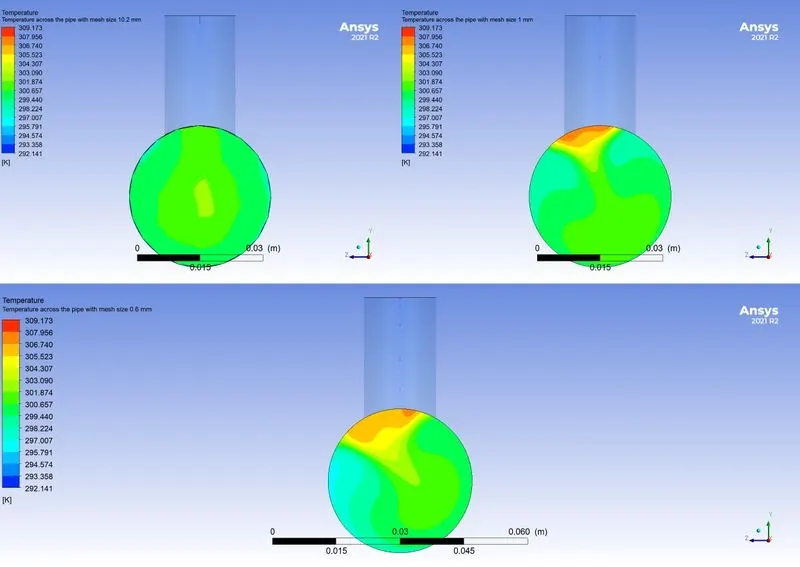
Comparision of Temperature across the pipe for three different mesh element size.	Comparision of Temperature across the pipe for three different mesh element size.
Momentum Ratio 4	Momentum Ratio 4
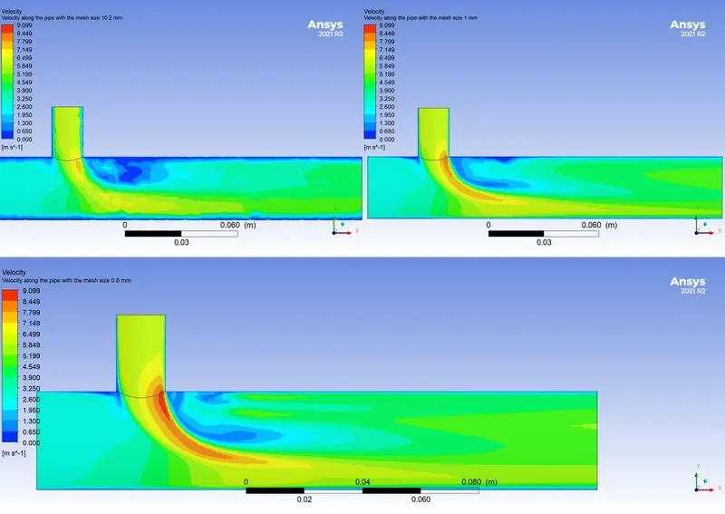
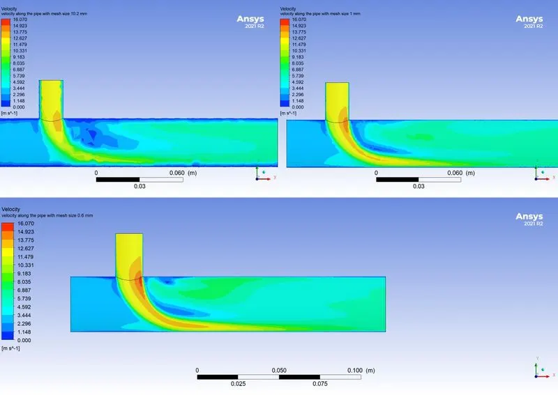
Comparision of Velocity along the pipe for three different mesh element size.	Comparision of Velocity along the pipe for three different mesh element size.
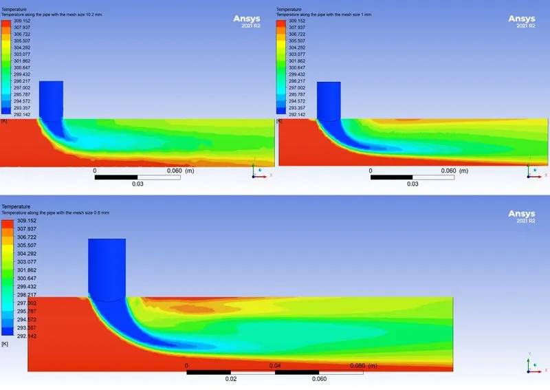
Comparision of temperature along the pipe with three different mesh element size	Comparision of temperature along the pipe with three different mesh element size
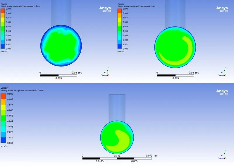
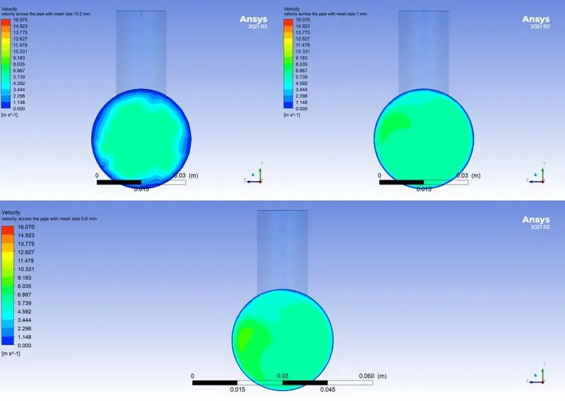
Comparision of velocity across the pipe with three different mesh element size.	Comparision of velocity across the pipe with three different mesh element size.
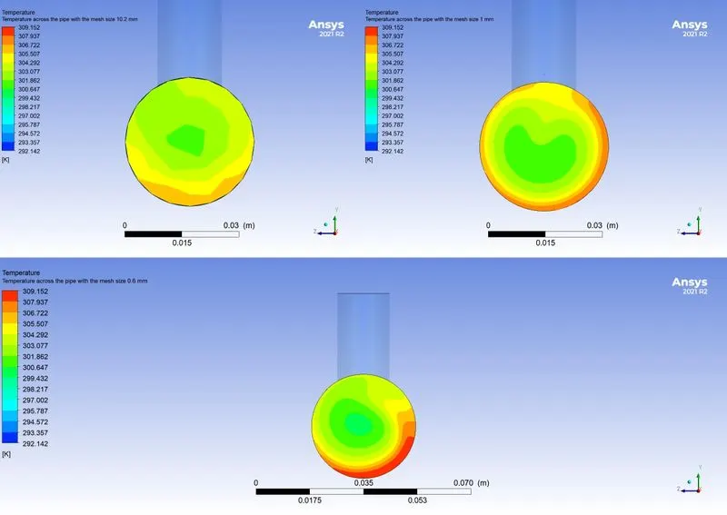
Comparision of temperature across the pipe with three different mesh element size.	Comparision of temperature across the pipe with three different mesh element size.

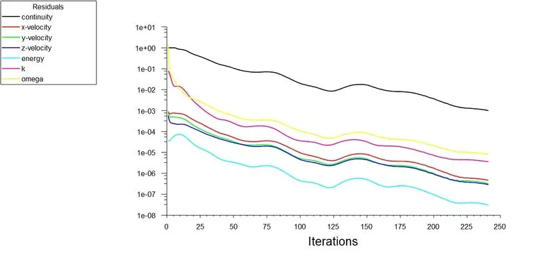
Convergence plot:

`K-epsilon` Realizable model:

Momentum ratio 2

i.Mesh Element size-10.2 mm

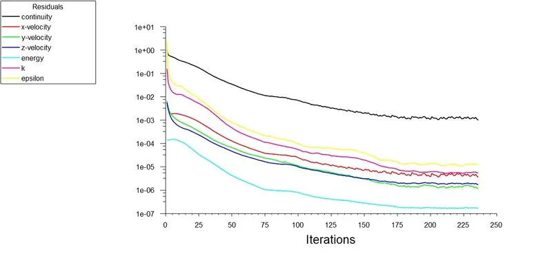
ii.Mesh Element Size-1 mm

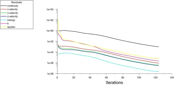
iii.Mesh Element Size-0.6 mm

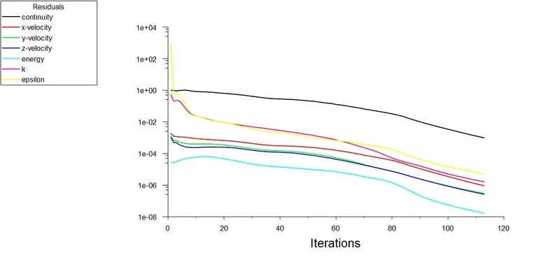
Momentum Ratio 4

iv.Mesh Element Size-10.2 mm

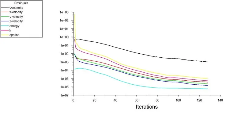
v.Mesh Element Size-1 mm

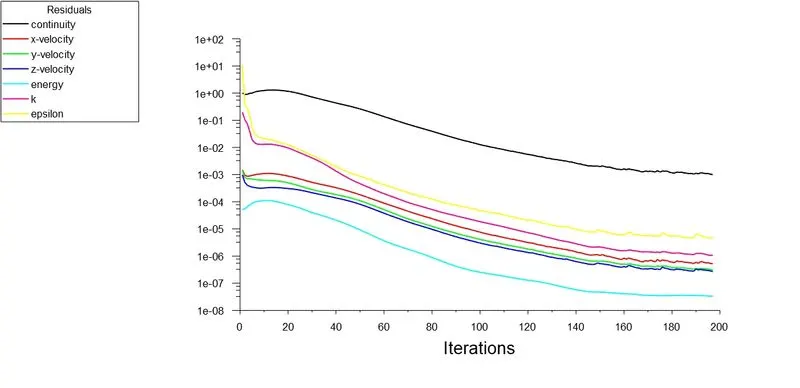
vi.Mesh Element Size-0.6 mm

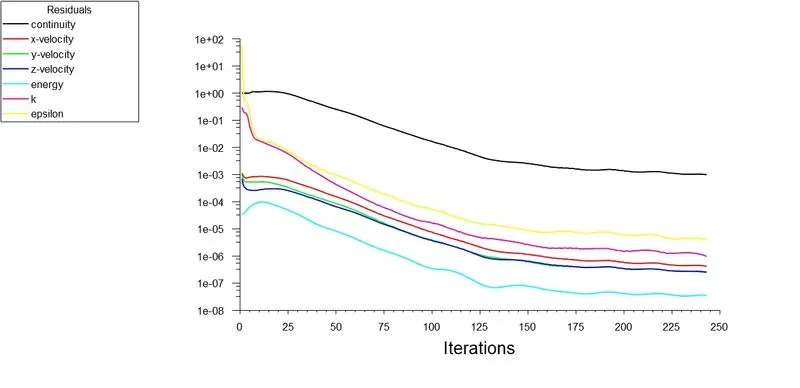
`K- omega` SST Model:

Momentum Ratio 2

vii.Mesh Element Size-10.2 mm

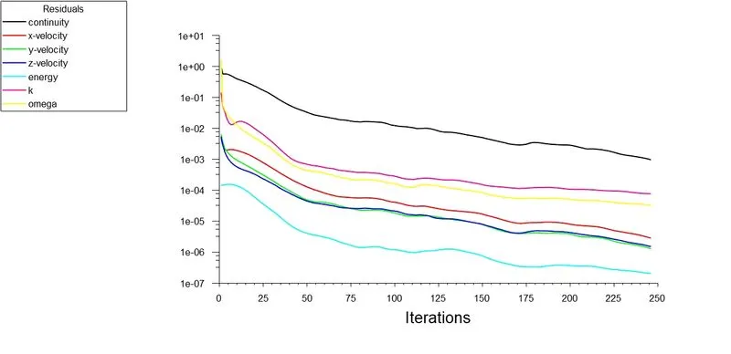
viii.Mesh Element Size-1 mm

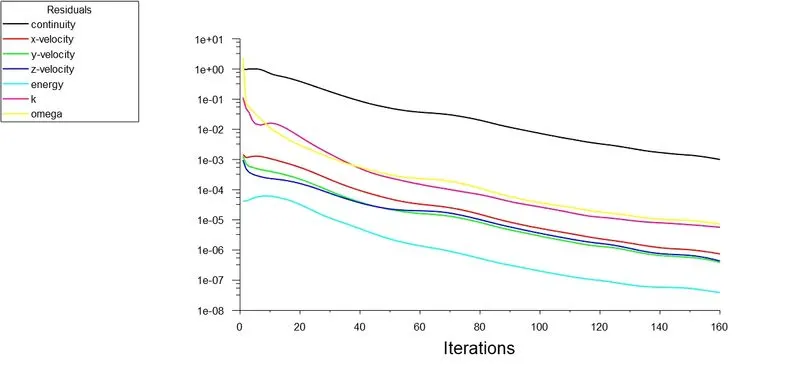
ix.Mesh Element Size-0.6 mm

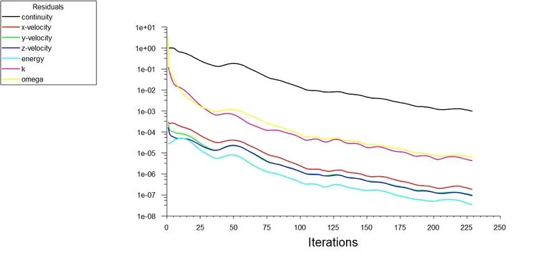
Momentum Ratio 4

x.Mesh Element Size-10.2 mm

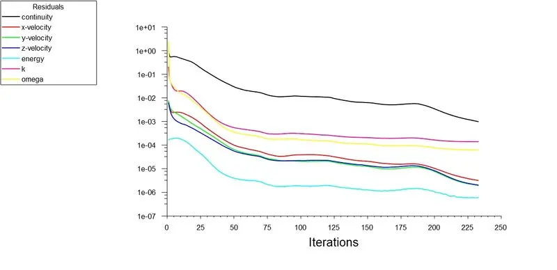
xi.Mesh Element Size-1 mm

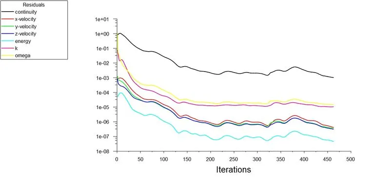
xii.Mesh Element Size-0.6 mm

	Mesh Size=0.0102 m				Mesh Size=0.001 m				Mesh Size=0.0006 m
	Momentum Ratio 2		Momentum Ratio 4		Momentum Ratio 2		Momentum Ratio 4		Momentum Ratio 2		Momentum Ratio 4
	K- Ѡ SST Model	K-ε realizable model	K -Ѡ SST Model	K-ε realizable model	K-Ѡ SST Model	K-ε realizable model	K -Ѡ SST Model	K-ε realizable model	K-Ѡ SST Model	K-ε realizable model	K -Ѡ SST Model	K-ε realizable model
No of iterations required for convergence	246	236	233	128	160	123	463	197	228	112	240	242
Standard Deviation	1.5500	1.5000	0.9500	1.0500	1.9000	1.7680	1.674	1.335	2.319	1.387	2.295	1.646
Average temperature outlet	30.258	30.227	27.506	27.528	30.500	30.425	27.578	27.542	30.500	30.450	27.703	27.580
Analytical Temperature	30.324	30.324	27.490	27.490	30.324	30.324	27.490	27.490	30.324	30.324	27.490	27.490
Error Percentage	0.21 %	0.31 %	0.05 %	0.13 %	0.58 %	0.33 %	0.32 %	0.18 %	0.58 %	0.41 %	0.77 %	0.32 %

Inference:

1. `K-epsilon`Realizable model converging faster compared to the `K-omega` SST model in most of the cases.

2. in most of the cases ,observe that increase in momentum ratio leads to decrease in standard deviation.

3. For a refined meshes `K- epsilon` Realizable model performed well.

4. eddies are mostly captured by `K- epsilon` Realizable model from plot.

5. Adapting a model based on the Less No.of.iterations for covergence and low error percentage in most cases.

6. `K-epsilon` Realizable Model will be opted as a viscous model.

Material Properties:

Air is used as the fluid to flow through the volume

Boundary Conditions:

constant velocity and temperature at inlets- hot inlet velocity is 3m/s and cold inlet velocity determined by momentum ratio. Temperature of hot inlet is 36 deg celcius and cold inlet 19 deg celcius

constant pressure at outlet - guage pressure is 0

walls with no-slip condition

Initialisation:

Hybrid initialisation is used to better guess the flow variables

Iterations increased to 20 to achieve a convergence

Run Calculation:

setting up a Simulations for 500 iterations.

Meshing:

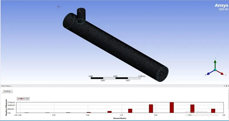
At first, Mesh indepenece study was conducted for the first case i.e ., Short tee pipe with two different ratios

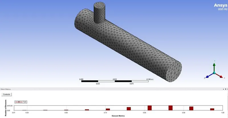
i.Short Tee - coarse Mesh (0.0102 m)

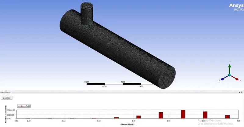
ii.Short Tee -intermediate Mesh (0.001 m)

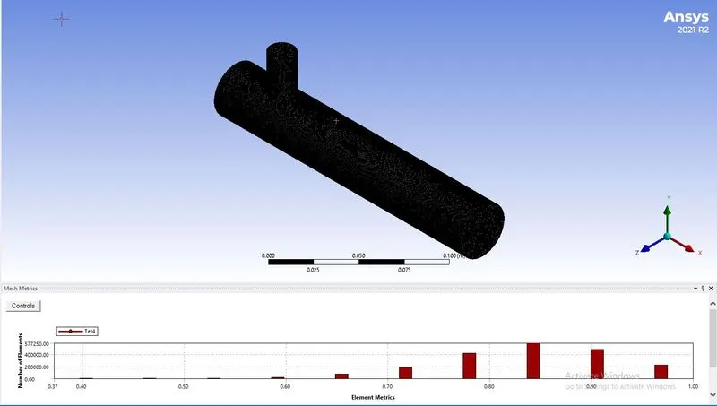
iii.Short Tee-Fine Mesh(0.0006 m)

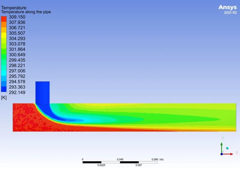
Our main parameter is Average temperature at outlet (it will provide that how well two different temperature fluids are mixed).

from the choosen viscous model, comparing the parameter

Mesh Sizes	Momentum Ratio 2-Average outlet temperature	Momentum Ratio 4-Average outlet temperature	Elements
0.0102 m (Coarse)	30.227	27.528	12556
0.001 m (Medium)	30.425	27.542	572772
0.0006 m (Fine)	30.450	27.580	1972728

From the table, observe that mesh is independent for the average outlet temperature with first decimal only

The medium and fine mesh (Average outlet temperature ) is independent on their mesh size.

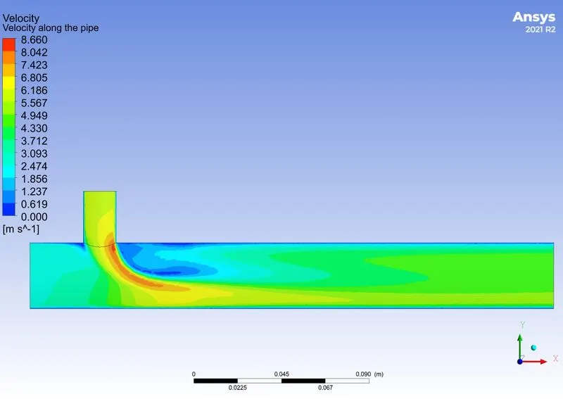
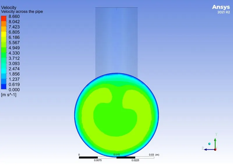
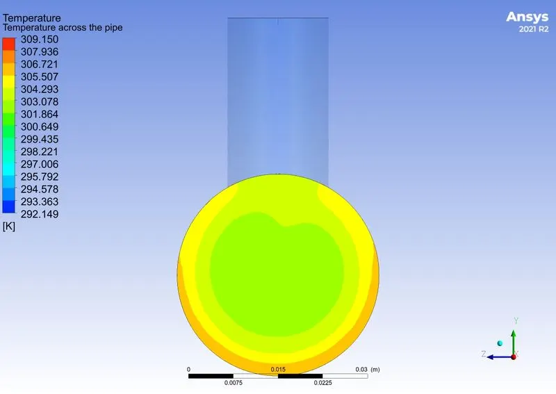
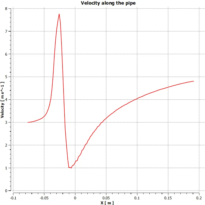
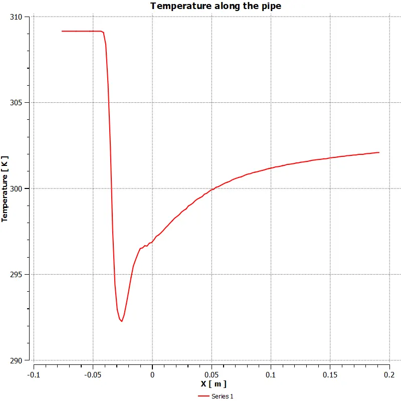
medium mesh and fine mesh shows a less difference in temperature and velocity at along and across the pipe when compared to coarse mesh ,it is clearly observed from the plots.

Long Tee Case setup:

i.Geometry - Long Tee pipe

ii.Mesh-mesh element size is 0.001 m,created named selection for boundaries

iii.Setup

solver type-pressure based

Solver time-steady

models-Energy equation is included,`K- epsilon` Realizable viscous model with standard wall functions is included.

cell Zones-Air as fluid used.

boundaries-given velocity 3m/s ,temperature -36 deg celcius as a input for inlet-X

velocity for cold inlet is determined based on the momentum ratio i.e., 2 and 4

velocity for cold inlet -6 m/s if momentum ratio is 2,veloocity for cold inlet is 12 m/s if momentum ratio is 4.

Velocity for cold inlet and temperature-19 deg celcius used as a input for inlet-Y

guage pressure-0,back pressure specification-Total pressure ,temperature - 26.85 deg celcius in outlet boundary

shear condition - no slip has used in walls condition

initialisation-hybrid is used.

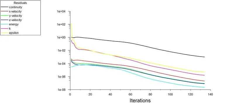
No of iterations under run calculation -500

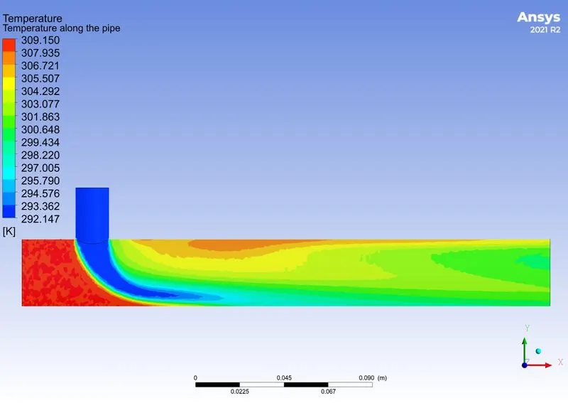
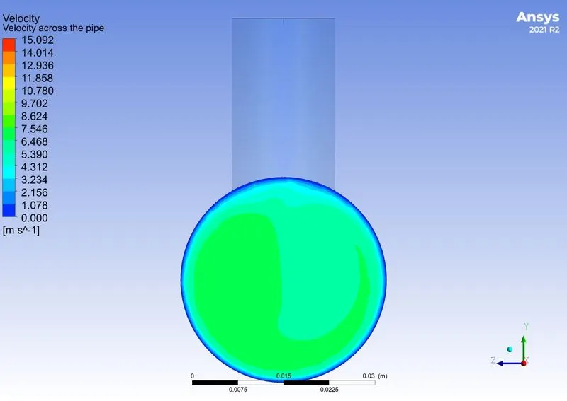
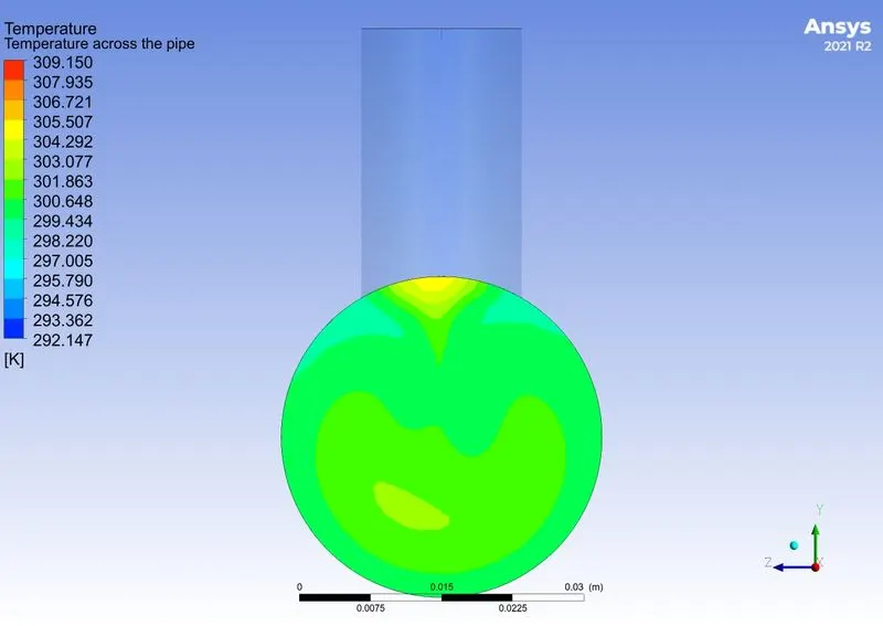
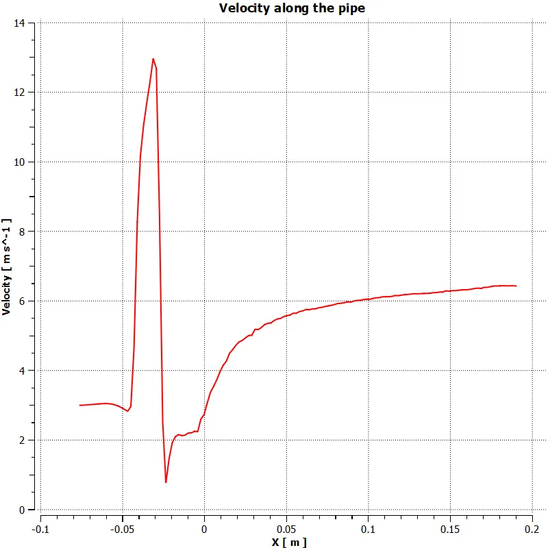
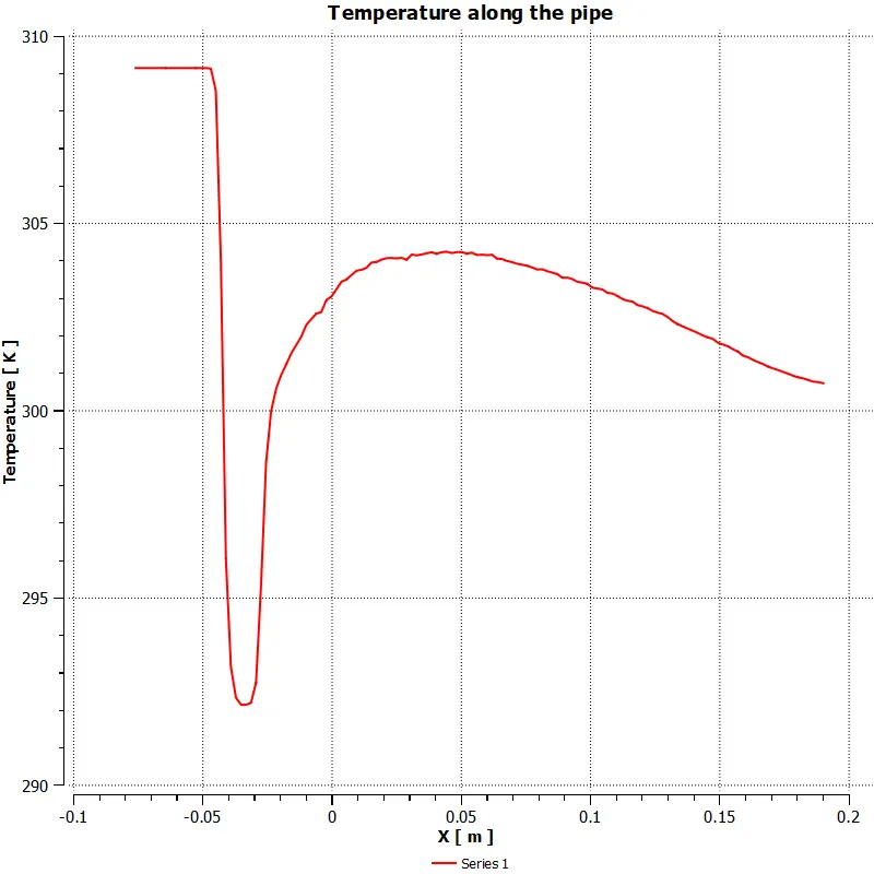
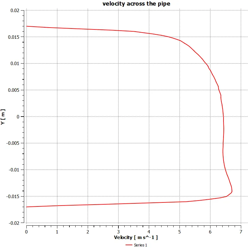
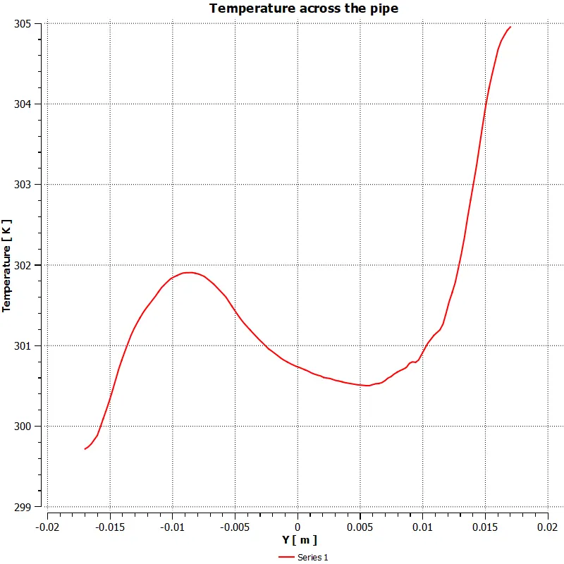
Case: Momentum Ratio 2

mesh

Plot:

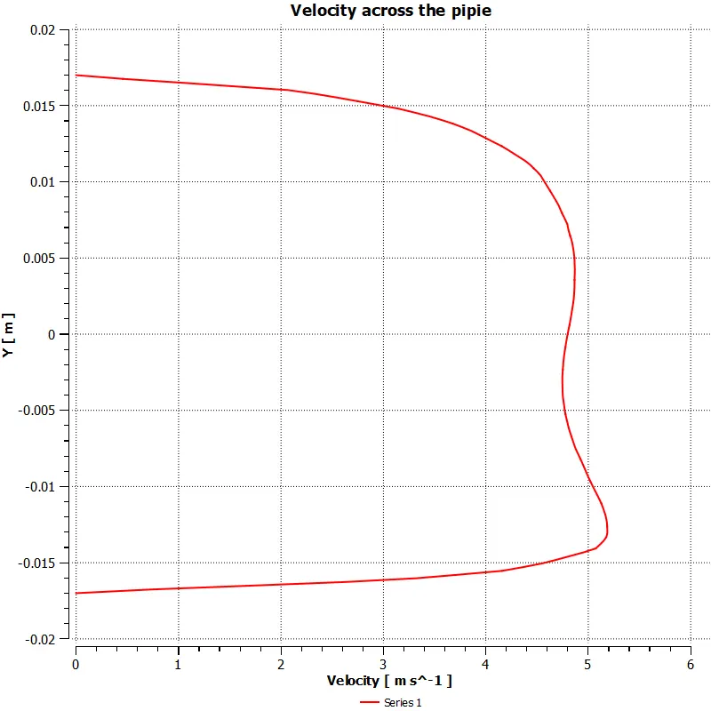
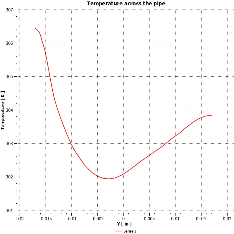
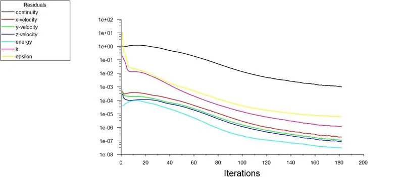
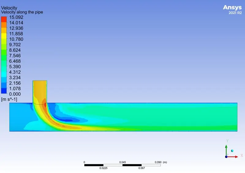
Case: Momentum Ratio 4

Conclusion:

Study has been carried out to determine the viscous model and mesh element size independent on the average outlet temperature and to visualise the steady state flow behaviour in the short Tee pipe.This study suggested `K- epsilon` realizable model and average outlet temperature independent from the mesh element size 0.001 m.

Another study conducted on the long tee pipe to visualise the steady state flow behaviour and to determine the mixing increases or not due to length by comparing with short tee pipe and comparing the momentum ratio's of 2 and 4 to estimate the mixing increase or not.This study suggests

	Cell Count	Average outlet Temperature	No of iterations for convergence
Short Tee,Momentum Ratio 2	572772	30.425	123
Short Tee,Momentum Ratio 4	572772	27.542	197
Long Tee,Momentum Ratio 2	754551	30.473	133
Long Tee,Momentum Ratio 4	754551	27.466	181

1.Increasing the length of Tee pipe doesnot improve the mixing effeciency.

2.Momentum ratio strongly influence the mixing efficiency because of turbulence characteristics.