Week 1- Mixing Tee
AIM:
To analyze the mixing in Tee-Joint as a result of different momentum ratios and length of the pipe using different RANS models and comparing results
Case -1: Short Tee with Momentum ratio = 2,4
Case -2: Long Tee with Momentum ratio = 2,4
GEOMETRY AND MESH:
- Used the Ansys Fluent module and imported the geometry
- Prepared the model for Fluent by extracting the volume inside
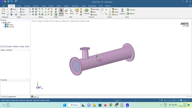
Fig1: Short Tee Model
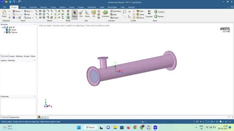
Fig2: Long Tee Model
- Suppressed the pipe for physics
- Added name tags to the inlets, outlet and wall appropriately
- Meshed the model using appropriate element size and checked for mesh quality
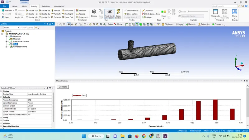
Fig3: Short Tee Mesh Quality
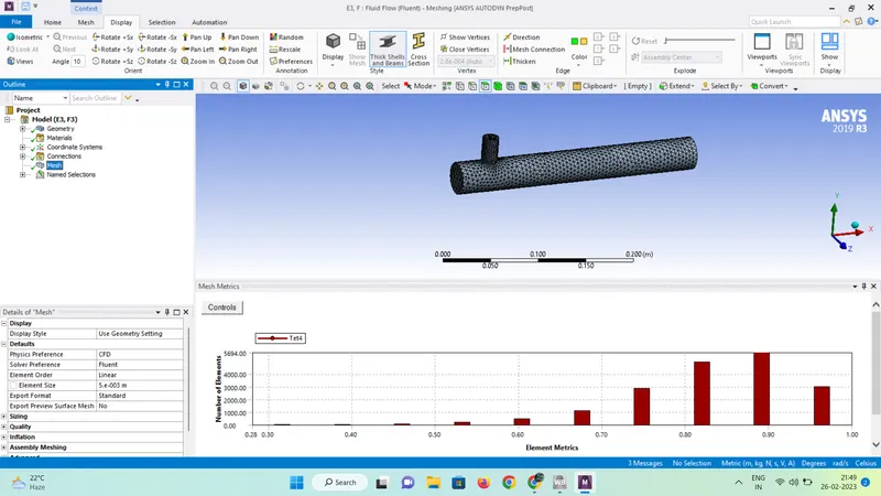
Fig4: Long Tee Mesh Quality
- Element size for both the cases is 0.005 mm
SET-UP :
- The standard property value for all the cases are as follows
| INLET-X TEMPERATURE | INLET-Y TEMPERATURE |
| 36 DEGREE CELCIUS | 19 DEGREE CELCIUS |
- Four set-ups are studied in this report given as follows
| CASE NO. | RANS MODEL | MOMENTUM RATIO | TEE-TYPE |
| CASE-1 | k-epsilon | 2 | SHORT |
| CASE-2 | k-epsilon | 4 | SHORT |
| CASE-3 | k-omega SST | 2 | SHORT |
| CASE-4 | k-omega SST | 4 | SHORT |
- By setting up the model for the above cases, the effect of the momentum ratio, length of the Tee and the model used for calculating turbulence is studied
RESULTS :
- The surface averaged temperature and standard deviation of the temperature at the outlet is used as a parameter to study convergence of the solution
- The convergence is determined by studying the following plots and contours
CASE -1
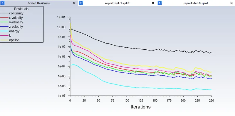
Fig5: Residuals for CASE-1
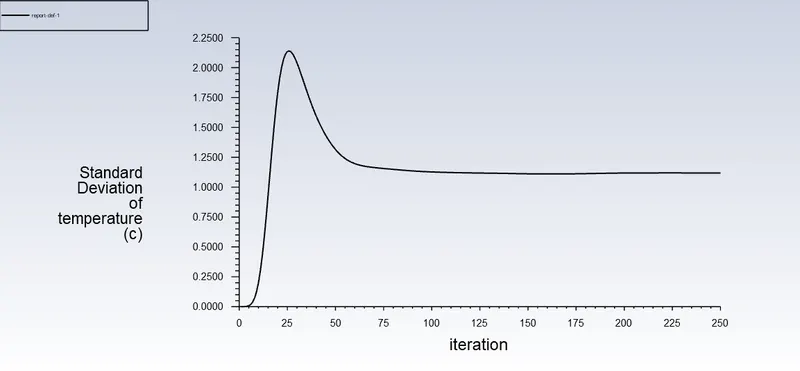
Fig6: Standard Deviation at outlet for CASE-1
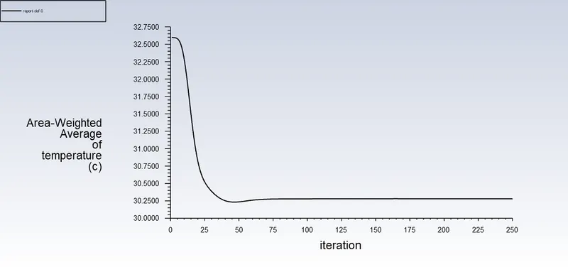
Fig7: Area Weighted average of temperature at outlet CASE-1
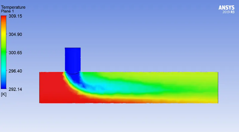
Fig8: Temperature Contour for CASE-1
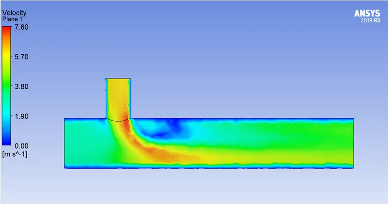
Fig9: Velocity Contour for CASE-1
CASE -2
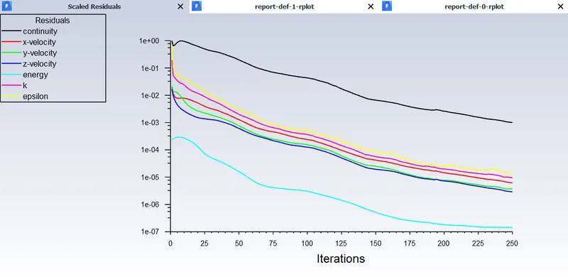
Fig10: Residuals for CASE-2
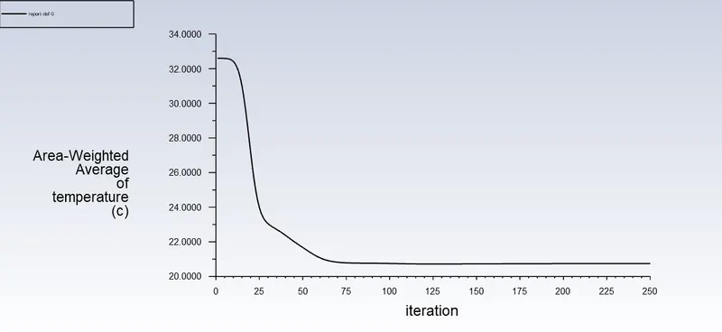
Fig11: Area Weighted average of temperature at outlet CASE-2
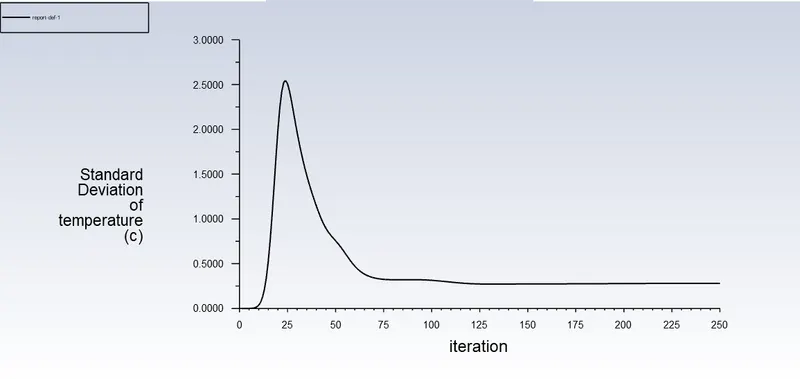
Fig12: Standard Deviation at outlet for CASE-2
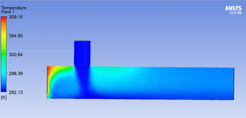
Fig13: Temperature Contour for CASE-2
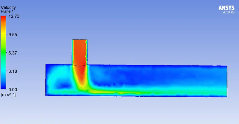
Fig14: Velocity Contour for CASE-2
CASE -3
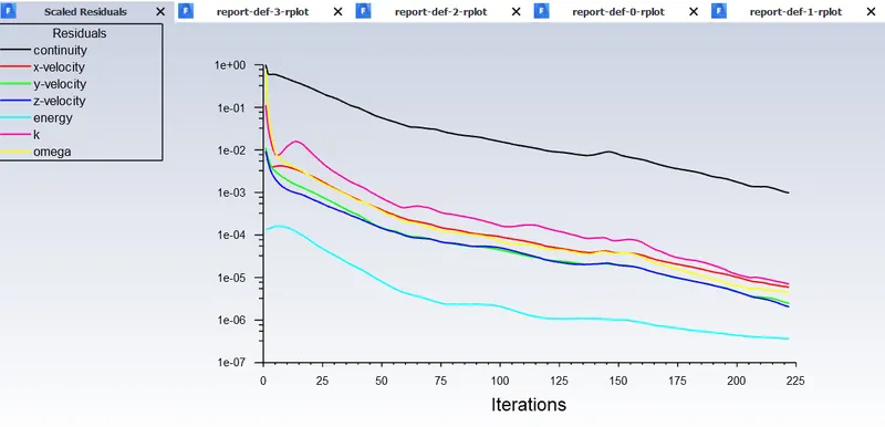
Fig15: Residuals for CASE-3
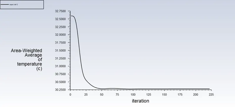
Fig16: Area Weighted average of temperature at outlet CASE-3
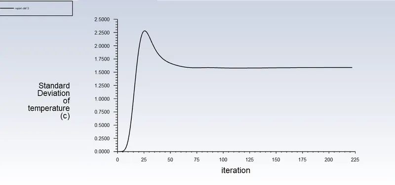
Fig17: Standard Deviation at outlet for CASE-3
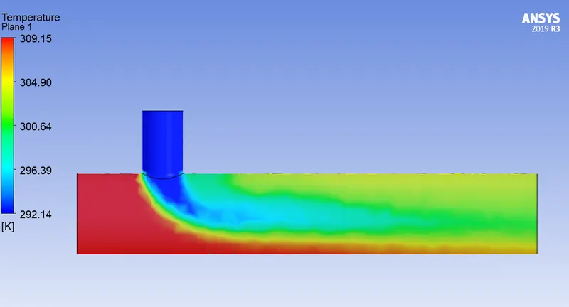
Fig18: Temperature Contour for CASE-3
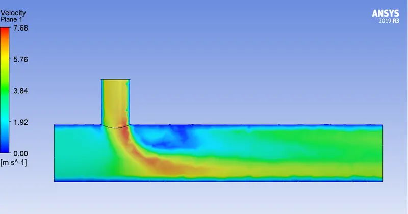
Fig19: Velocity Contour for CASE-3
CASE -4
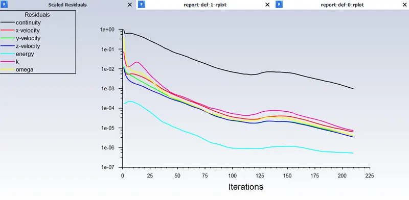
Fig20: Residuals for CASE-4
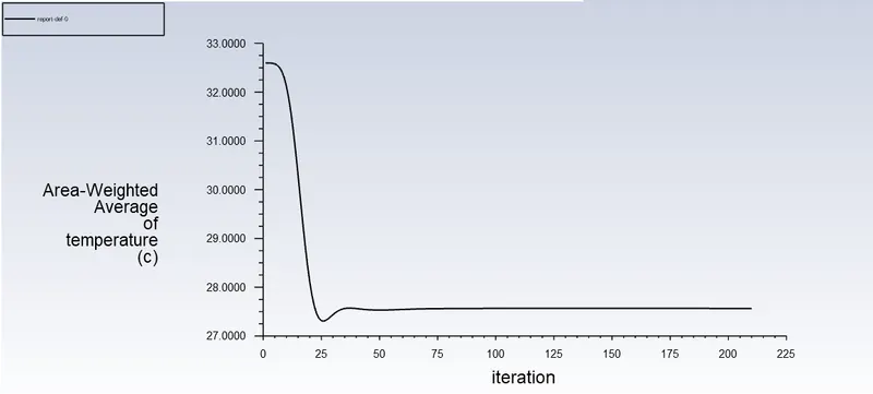
Fig21: Area Weighted average of temperature at outlet CASE-4
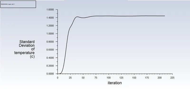
Fig22: Standard Deviation at outlet for CASE-4
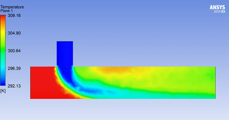
Fig23: Temperature Contour for CASE-4
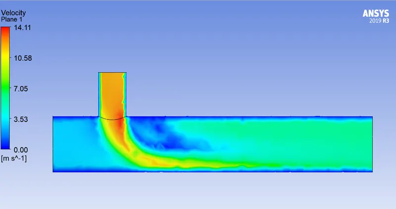
Fig24: Velocity Contour for CASE-4
COMPARISON TABLE FOR SHORT TEE RESULTS
| Momentum Ratio | Model | Average Outlet Temp | Temp Standard Deviation | Analytical Temp of mixture |
| 2 | k-epsilon | 30.25 | 1.2 | 30.3 |
| 4 | k-epsilon | 21 | 0.25 | 27.5 |
| 2 | k-omega SST | 30.25 | 1.55 | 30.3 |
| 4 | k-omega SST | 27.50 | 1.4 | 27.5 |
- By comparison table shown above, it can be clearly seen that the simulation results don't match the analytical results in the case of k-epsilon model in the case on larger momentum ratio
CHOICE OF MODEL FOR LONG TEE
- The k-epsilon and k-omega SST models are from the RANS ( Reynolds Averaged Navier Stokes) category. Both of the models are 2 eqn models which focus on the modeling of Reynolds stresses by using equations for the closure of the Reynolds Averaged equations.
- It is observed in the above data that k-omega SST model captures the physics of the mixing tee in a more accurate manner
- The k-epsilon model is usually used for solving external flows and k-omega model is used for solving internal flows.
Due to these reasons, k-omega SST model is used to study the results and effects of using a long tee for mixing
LONG TEE SET-UP
| CASE NO. | RANS MODEL | MOMENTUM RATIO | TEE-TYPE |
| CASE-5 | k-omega SST | 2 | LONG |
| CASE-6 | k-omega SST | 4 | LONG |
RESULTS
CASE-5
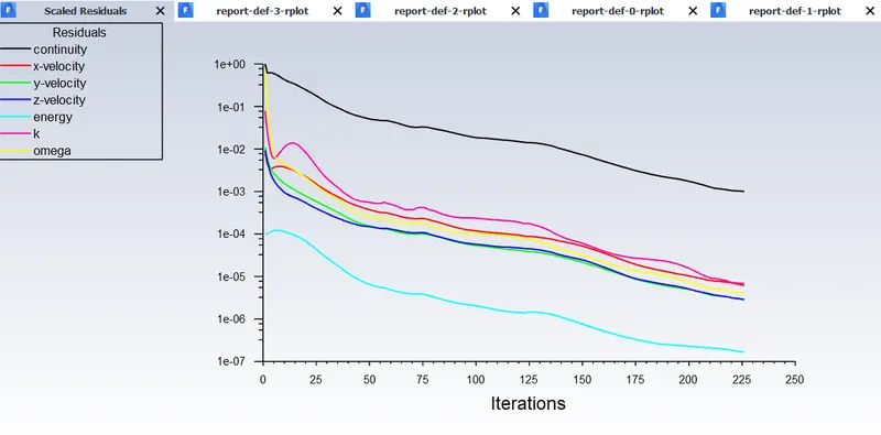
Fig25: Residuals for CASE-5
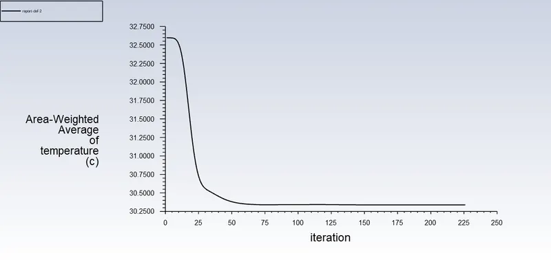
Fig26: Area Weighted average of temperature at outlet CASE-5
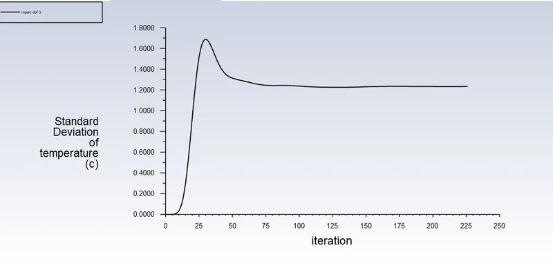
Fig27: Standard Deviation at outlet for CASE-6
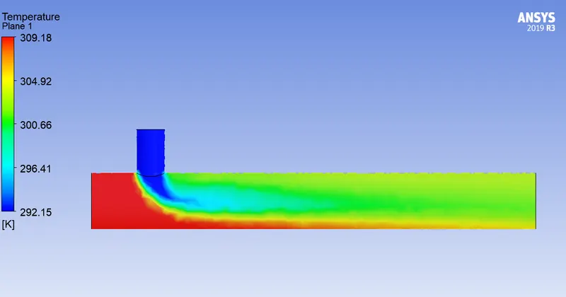
Fig28: Temperature Contour for CASE-5
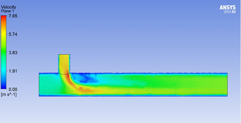
Fig29: Velocity Contour for CASE-5
CASE-6
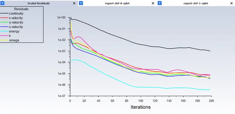
Fig30: Residuals for CASE-6
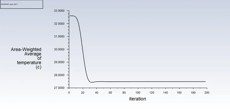
Fig31: Area Weighted average of temperature at outlet CASE-6
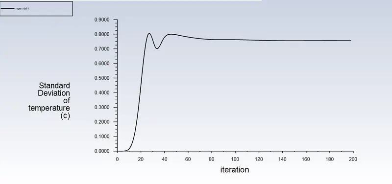
Fig32: Standard Deviation at outlet for CASE-6
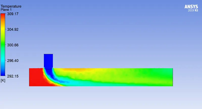
Fig33: Temperature Contour for CASE-6
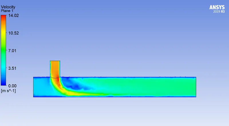
Fig34: Velocity Contour for CASE-6
COMPARISON BETWEEN LONG AND SHORT TEE
| CASE TYPE | MOMENTUM RATIO | CELL COUNT | TEMP STANDARD DEVIATION | AVERAGE OUTLET TEMP. | ITERATIONS FOR CONVERGENCE |
| SHORT | 2 | 14330 | 1.55 | 30.25 | 225 |
| SHORT | 4 | 14330 | 1.4 | 27.5 | 215 |
| LONG | 2 | 18175 | 1.2 | 30.25 | 225 |
| LONG | 4 | 18175 | 0.75 | 27.5 | 200 |
- The data shows that the average temperature at the outlet is independent of the tee length, but the standard deviation is lesser for long tee
MESH INDEPENDENCE TEST
A method of determining if the simulation results are independent of the underlying mesh is to conduct a mesh independence study. You accomplish this by running several simulations with various mesh resolutions and observing whether the outcomes change.
| MESH SIZE | CELL COUNT | AVERAGE OUTLET TEMP | TEMP STANDARD DEVIATION |
| 0.005 | 14330 | 27.5 | 1.4 |
| 0.01 | 12740 | 27.5 | 1.4 |
| 0.5 | 8839 | 27.5 | 1.4 |
Here as the outcomes do not change with the mesh, it can be concluded that this simulation is mesh independent