Week 1- Mixing Tee

Aim:-

To create a two versions of the mixing tee. One of them is longer than the other.

Your job is to set up steady-state simulations to compare the mixing effectiveness when hot inlet temperature is 36⁰C & the Cold inlet is at 19⁰C.

Use the k-epsilon and k-omega SST model for the first case and based on your judgment use the more suitable model for further cases. Giving the reason for choosing a suitable model is compulsory.

1. Case 1
   • Short mixing tee with a hot inlet velocity of 3m/s.
   • Momentum ratio of 2, 4.
2. Case 2
   • Long mixing tee with a hot inlet velocity of 3m/s.
   • Momentum ratio of 2, 4.

Momentum ratio = velocity at cold inlet / velocity at hot inlet

In a table, compare the following values from the 2 cases.

1. Cell count
2. Average outlet temperature
3. Number of iterations for convergence

Expected results:

1. Velocity and temperature contour plots on the cut planes along and across the pipe.
2. Velocity and temperature line plots along and across the length of the pipe.
3. Perform Mesh independent study for any one case.
4. Discuss the effect of length and momentum ratio on results.

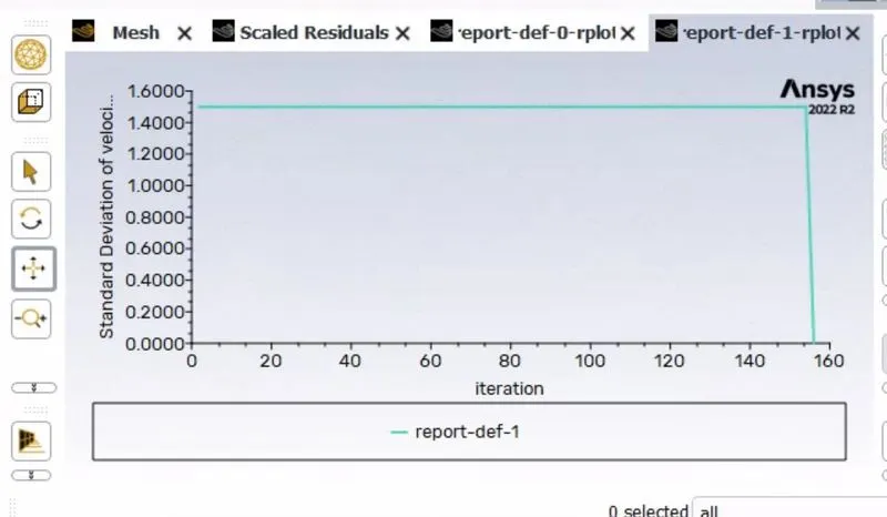
For each simulation, you need to show the convergence plot.

Introduction:-

Mixing tees are commonly used in the petrochemical industry to blend two fluid streams with different physical and/or chemical properties. Temperature fluctuations in the metal may cause thermal fatigue in the pressure boundary pipes. If there is through-wall cracking, the fluid may leak, causing a fire and other hazards. As a result, it is critical to ensure that temperature differences are kept to a minimum so that the pipe system can withstand them. Redesigning the pipe system so that the momentum ratio of the two fluid streams is advantageous for rapid mixing is one option, as is installing systems that protect the pressure boundary piping to improve mixing and prevent temperature swings.

Theory:-

In this tee junction simulation, the same fluid is mixed at varied temperatures and inlet velocities through two perpendicular inlet pipes to calculate temperature change. The simulation is repeated twice, with the only variable being the geometry length (one is shorter than the other). Furthermore, for each example, we will simulate for momentum ratios of 2 and 4.
The k-"> and k-"> SST models are employed for the first example, and the more appropriate model is utilised for subsequent cases based on the decision.
The k-epsilon model is best suited for flow away from the wall, such as free surface flow.
The k-omega model is best suited for near-wall-flow regions where an unfavourable pressure gradient develops.

Three steps are required to analyse a problem using the CFD technique:

Primary Processing

Solving

Post-Processing

Preprocessing entails preparing the geometry model for the required simulation. The geometry is imported here, the fluid volume is calculated, and several further processes are taken. Following that, the model is suitably meshed.

Solving entails using applicable initial circumstances, boundary conditions, turbulence models, and so on.

Postprocessing:This phase is used to analyse the results obtained in the solution and allows for a more understanding representation of the results.

Procedure:-

The procedure begins with configuring the project site by dragging and dropping the fluent icon into the project schematic window, as shown below.
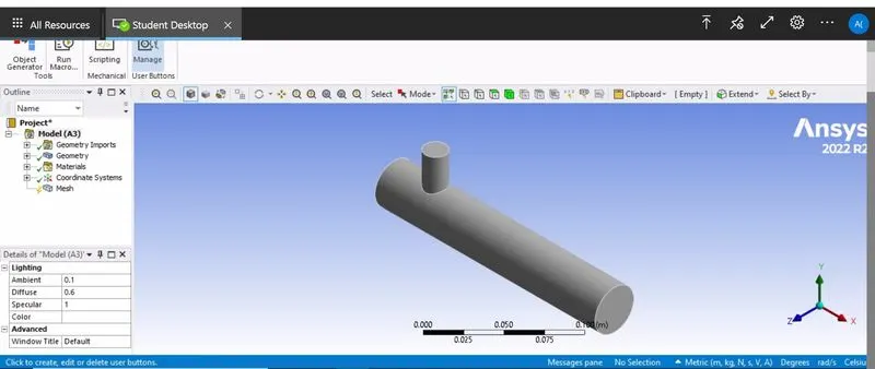
The cad file will be imported from the directory into the geometry menu, where we will use spaceclaim to clean up the geometry, as shown below.
In spaceclaim, the imported geometry looks like this. To remove the edges and ensure that only the volume through which the fluid moves remains, go to the prepare menu and select the Volume extract option, as shown below.
Right-click shell1 in the structure tree and select the'suppress for physics' option. This ensures that only the blue-colored element is left intact for analysis.

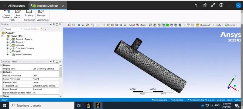
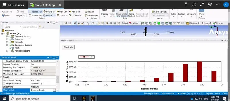
This is how the tree is updated. Double-click on the mesh to open a window.
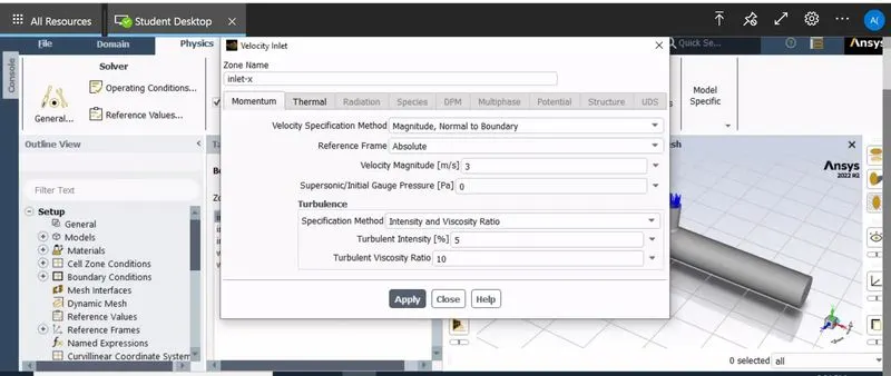
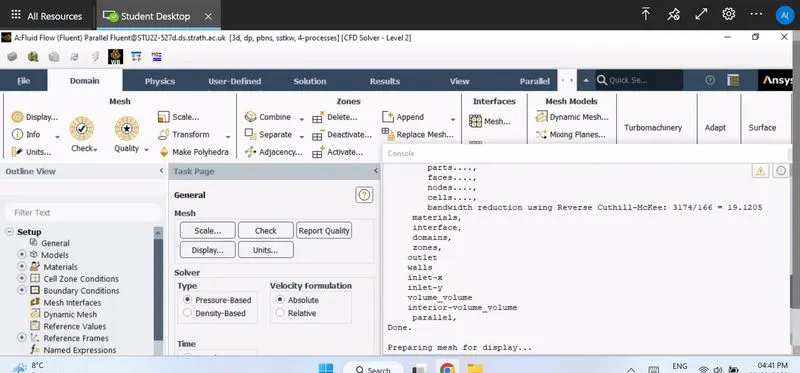
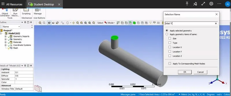
Once the meshing is complete, the next step is to provide the solver with initial values and boundary conditions by specifying them in the setup menu. Double-click it.
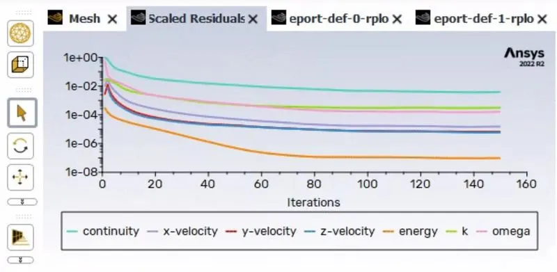
Because fluids of different temperatures are mixing, select the energy equation. Then, in the menu, specify the boundary conditions as specified in the challenge, and run the solution for 150 iterations before repeating the steps for different cases.

Solution:-

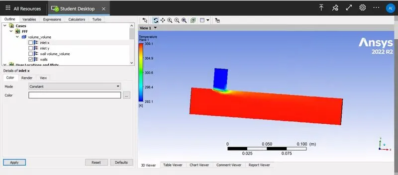
For a Short mixing tee of momentum ratio 2 and 4:

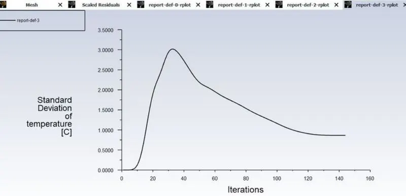
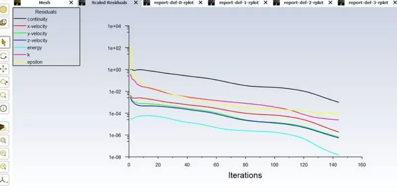
Long mixing tee for momentum ration 2 and 4:

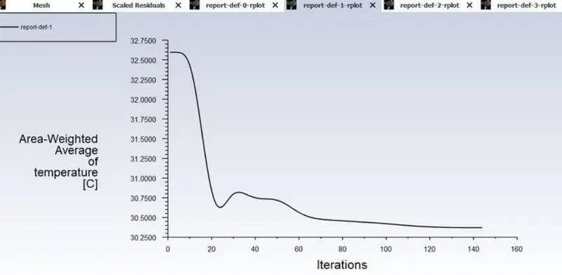
Result:-

Cases Cell count Average outlet temperature (K) Number of iterations for convergence
Case 1 Short-T (momentum ratio=2) 564818 309 138
Case 1 Short-T (momentum ratio=4) 564818 292 170
Case 2 long-T (momentum ratio=2) 755032 309 144
Case 2 long-T (momentum ratio=4) 755032 292 606

Conclusion:-

The combined air's outlet temperature demonstrates that as the momentum ratio increases, so does the mixing efficiency. As the momentum ratio increases, so does the cold inlet velocity, which aids in better mixing of the fluids in the pipe.
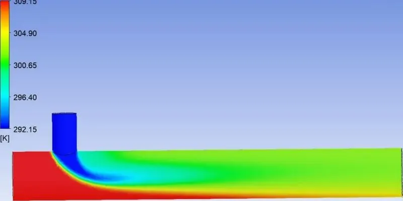
The temperature contours of short-T and Long-T with momentum ratios of 2 and 4 show that as the length of the mixing-T increases, so does the mixing effectiveness. As a result, Long-T has a uniform temperature drop at the outlet.

References:-

Th. Frank, C. Lifante, H.-M. Prasser, F. Menter,
Simulation of turbulent and thermal mixing in T-junctions using URANS and scale-resolving turbulence models in ANSYS CFX,
Nuclear Engineering and Design,
Volume 240, Issue 9,
2010,
Pages 2313-2328.

Thanks