Week 1- Mixing Tee

AIM

• To set up steady-state simulations to compare the mixing effectiveness when hot inlet temperature is 36⁰C & the Cold inlet is at 19⁰C.
• To conduct a mixing Tee simultaion for 2 different lengths of pipe:
• Case 1
  • Short mixing tee with a hot inlet velocity of 3m/s.
  • Momentum ratio of 2, 4.
• Case 2
  • Long mixing tee with a hot inlet velocity of 3m/s.
  • Momentum ratio of 2, 4.
• Momentum ratio = velocity at cold inlet / velocity at hot inlet

• Compare the following values from the 2 cases using a table

  1. Cell count
  2. Average outlet temperature
  3. Number of iterations for convergence
• Obtain velocity and temperature contour plots on the cut planes along and across the pipe.
• Obtain velocity and temperature line plots along and across the length of the pipe.
• Perform Mesh independent study for any one case.
• Discuss the effect of length and momentum ratio on results.

INTRODUCTION

• In the petrochemical sector, mixing tees are widely used to combine two fluid streams with various physical and/or chemical qualities. The pressure boundary pipes may get thermally fatigued as a result of temperature changes in the metal. The fluid may leak if there is through-wall cracking, which could result in a fire and other problems. Therefore, it is crucial to ensure that temperature variations are minimal enough for the pipe system to endure them. Options include redesigning the piping system so that the momentum ratio of the two fluid streams is favorable for rapid mixing or installing mechanisms that safeguard the pressure boundary piping to improve the mixing of the two streams and reduce temperature swings.

THEORY

• The same fluid is mixed at various temperatures and inlet velocities through two perpendicular inlet pipes in this tee junction simulation to calculate the change in temperature. The simulation is run twice, with the sole difference between the cases being the geometry length (one is shorter than the other). Furthermore, we will simulate for momentum ratios of 2 and 4 for each case.
• k-ε">k-ε and k-ω">k-ω SST model are used for the first case and based on the judgment, the more suitable model is used for further cases.
• k-epsilon model: k-epsilon is best suited for flow away from the wall for example free surface flow region.
• k-omega model: k-omega is best suited for near the wall-flow region where the adverse pressure gradient is developed.
• SST(Shear stress transport) k-omega model: it is a 2 equation eddy viscosity model. it is a hybrid model combining the Wilcox k-omega and k-epsilon.

SOLVING AND MODELLING APPROACH

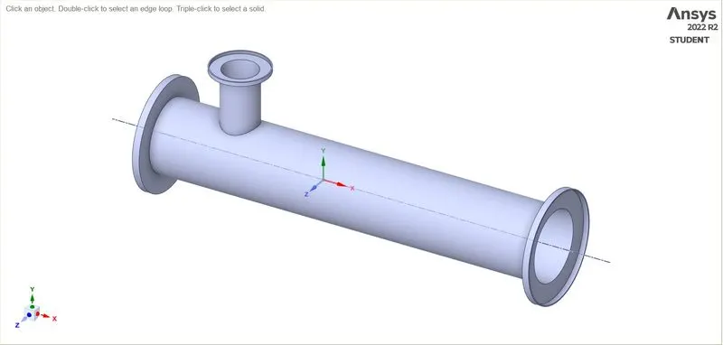
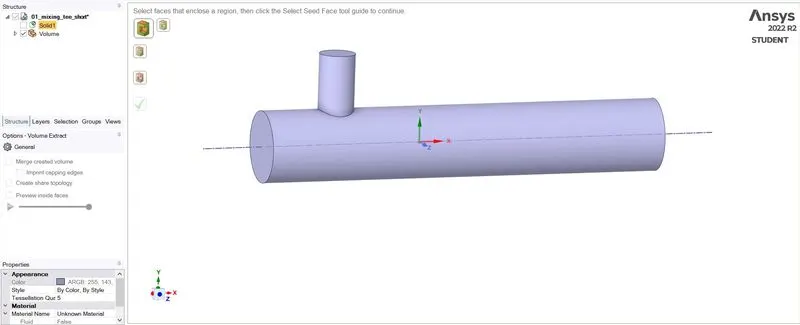
• Mixing-Tee model simulation requires only the fluid volume not the solid volume. Hence the fluid volume is extracted and then further simulations are done on the required fluid volume.
• The required fluid volume is then meshed.
• k-ε">k-ε and k-ω">k-ω SST model can be used for simulations.
• Mixing-Tee geometry and the required fluid volume is shown in the figures below.

PRE-PROCESSING AND SOLVER SETTING

1.Geometry

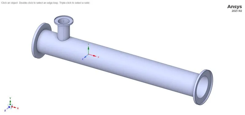
• Short Mixing-Tee and Long mixing-Tee geometry is shown in the figures below.

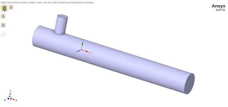
• Short mixing-Tee and Long mixing-Tee extracted fluid volume model is shown in the figures below.

2.Mesh

2.1. Mesh independency test

• Mesh independency test is conducted on short mixing-Tee

Mesh	Mesh elements
Coarse	12680
Medium	39097
Fine	564818

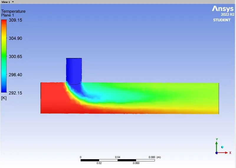
• Temperature distribution contour for coarse mesh is shown in the figure below.

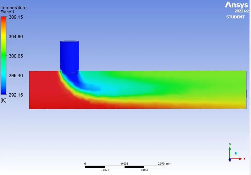
• Temperature distribution contour for Medium mesh is shown in the figure below.

• Temperature distribution contour for Fine mesh is shown in the figure below.

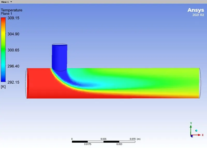
• When the three temperature distribution contours are compared, the fine meshed contour shows smooth mixing interphase of fluids of two different temperatures than the coarse and medium mesh temperature contours. Hence further simulations is carried out using the fine mesh in both the cases of mixing-Tee.

2.2. Case 1: Short mixing-Tee

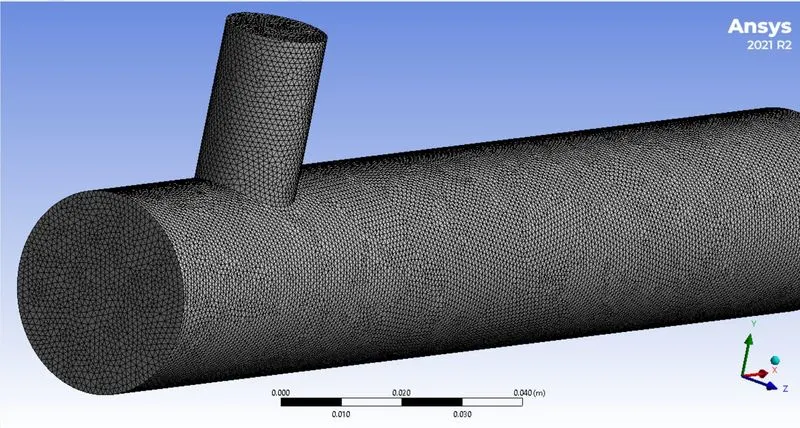
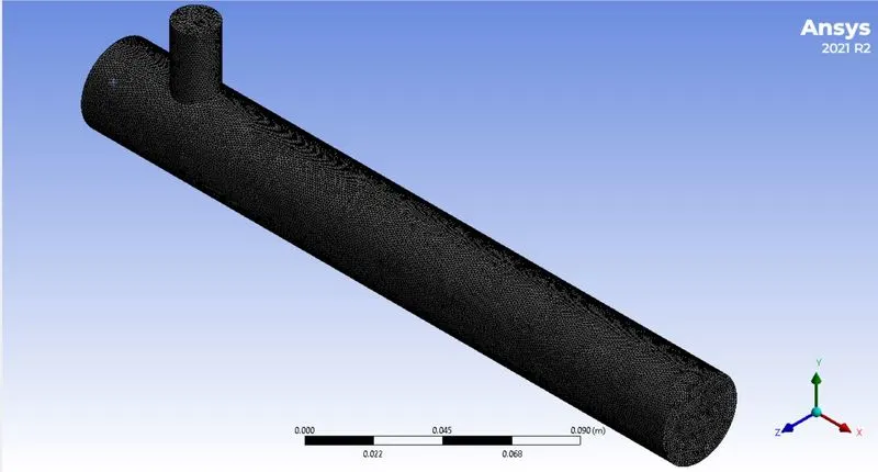
• Short mixing-Tee mesh model is shown in the figure below.

• Long mixing-Tee mesh model is shown in the figure below.

3. Solver requirements

3.1 Model choosed

• Here k-epsilon model is used , since flow mixing is happening away from the walls of the pipe. Hence this model is used for every calculations in this simulation

3.2 Boundary conditions

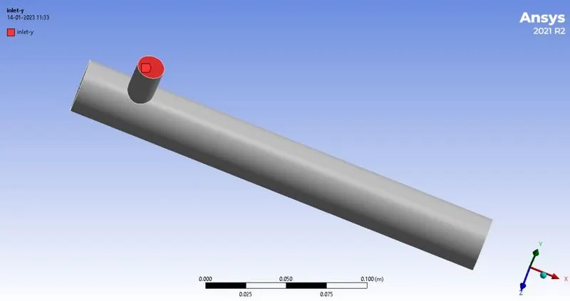
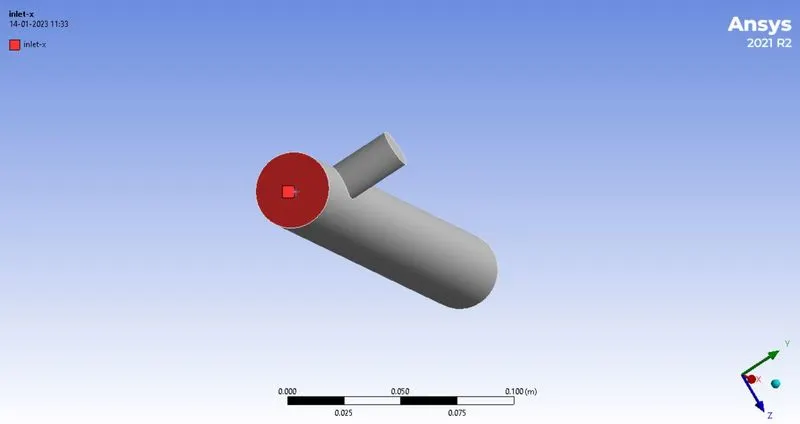
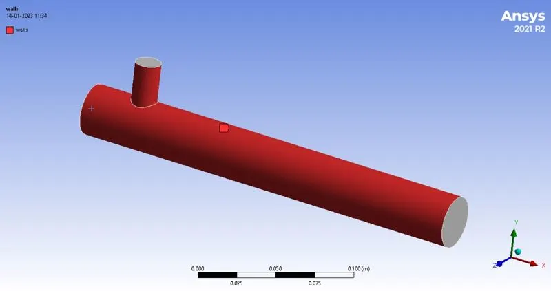
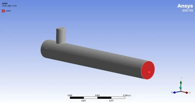
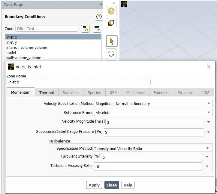
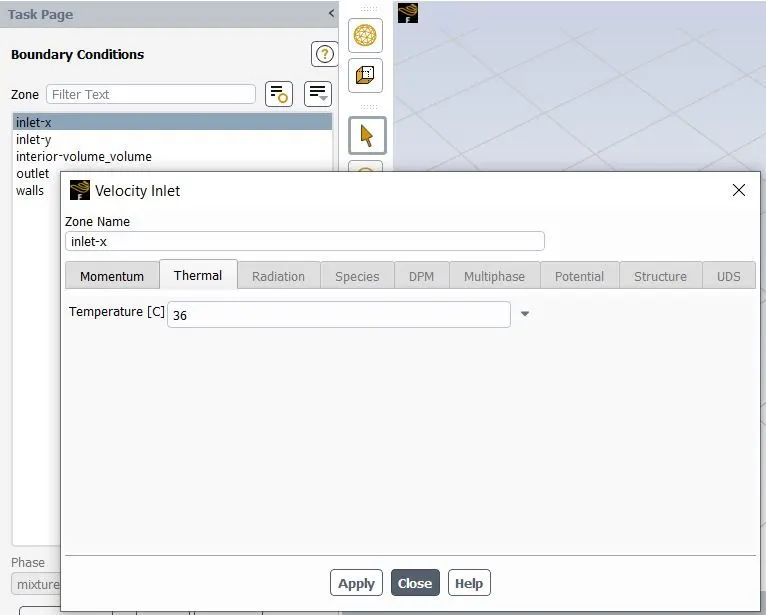
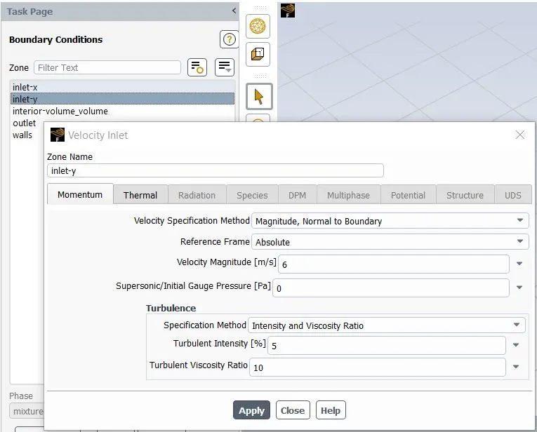
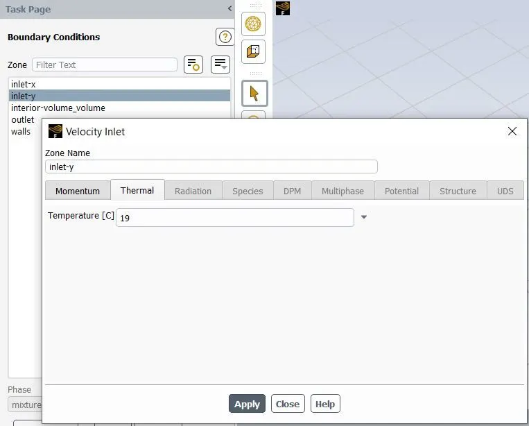
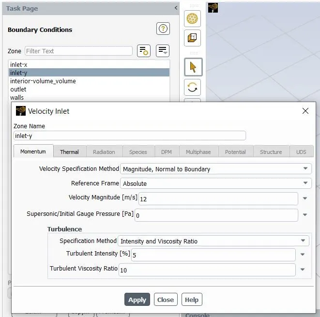
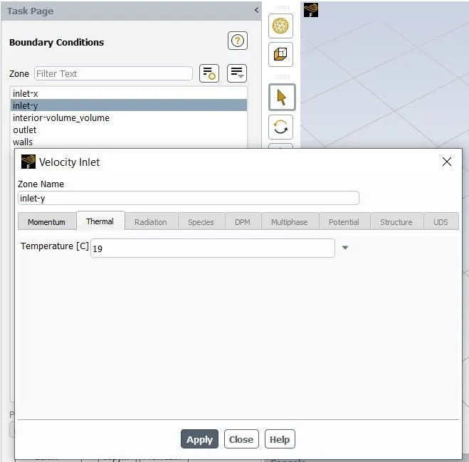
• Asigned boundary conditions for both Short mixing-Tee and Long mixing-Tee is shown shown in the figures below.

Inlet-y

Inlet-x

Walls

Outelt

Short mixing-Tee and Long mixing-Tee with momentum ratio = 2

• Hot inlet velocity = 3 m/s
• Hot inlet temperature = 36⁰C

• Cold inlet velocity = 6 m/s
• Cold inlet temperature = 19⁰C

Short mixing-Tee and Long mixing-Tee with momentum ratio = 4

• Hot inlet velocity = 3 m/s
• Hot inlet temperature = 36⁰C

• Cold inlet velocity = 12 m/s
• Cold inlet temperature = 19⁰C

RESULTS

Short mixing-Tee with momentum ratio = 2

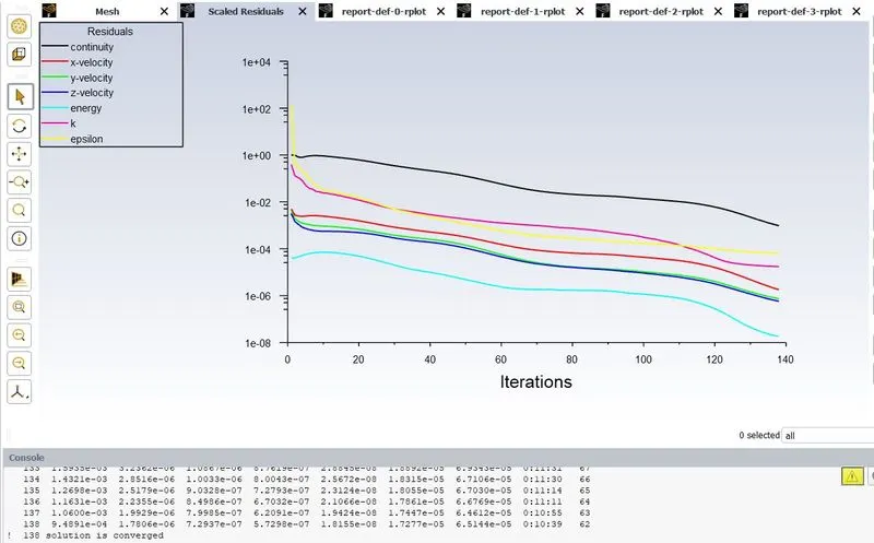
• Residual plot

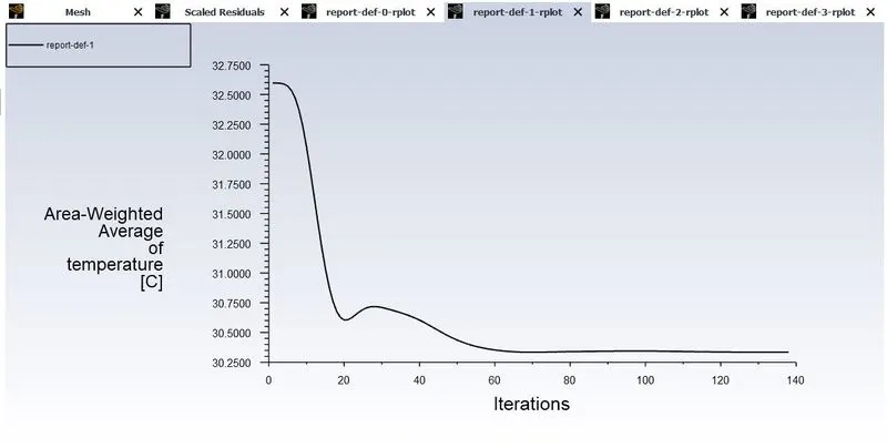
• Area weighted average of temprature at outlet for each iteration

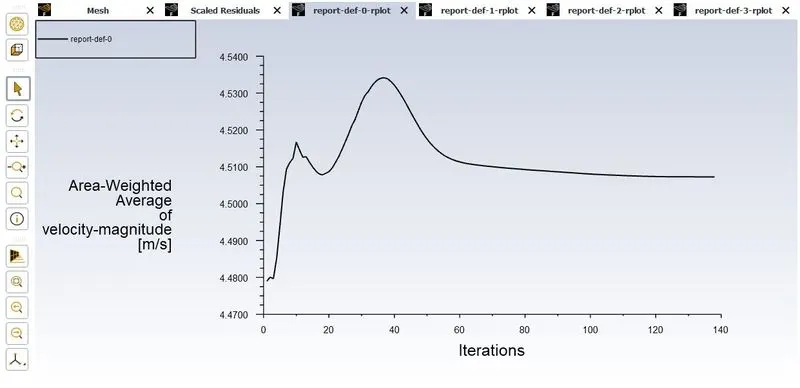
• Area weighted average of velocity at outlet for each iteration

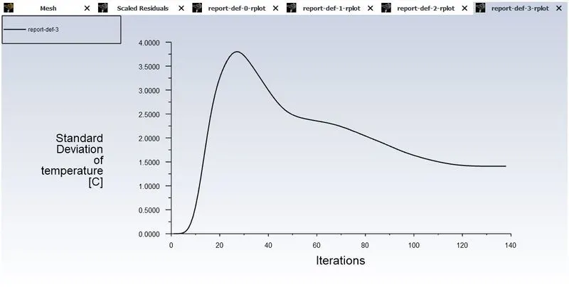
• Standard deviation of temprature at outlet for each iteration

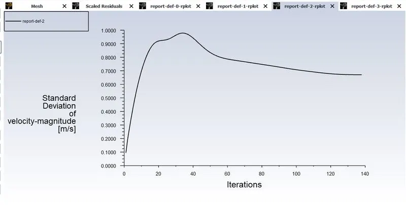
• Standard deviation of velocity at outlet for each iteration

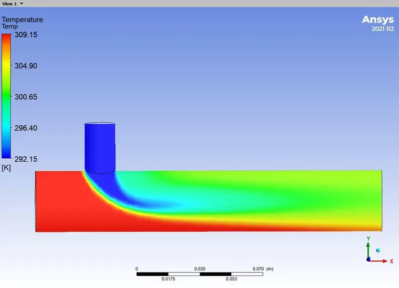
• Temperature contour

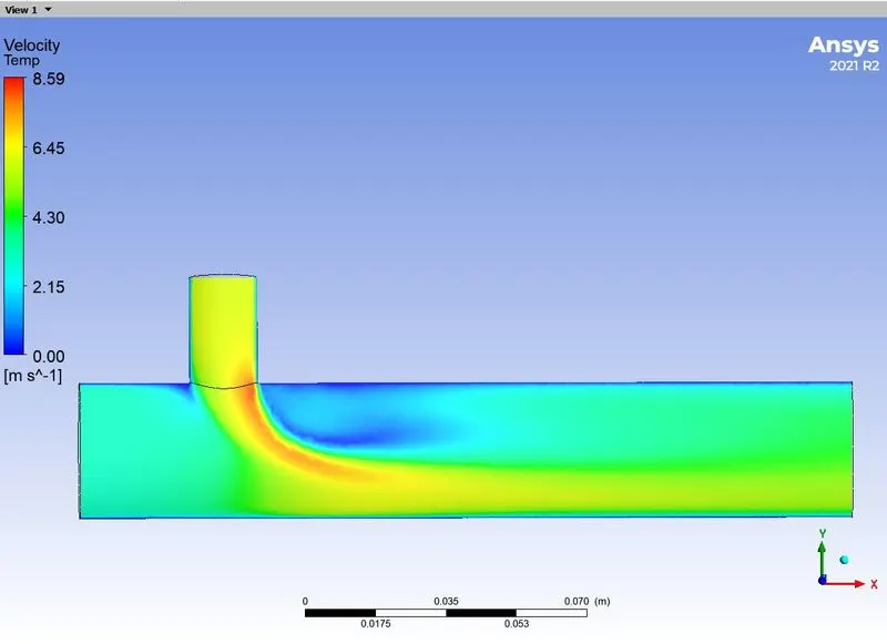
• Velocity contour

Short mixing-Tee with momentum ratio = 4

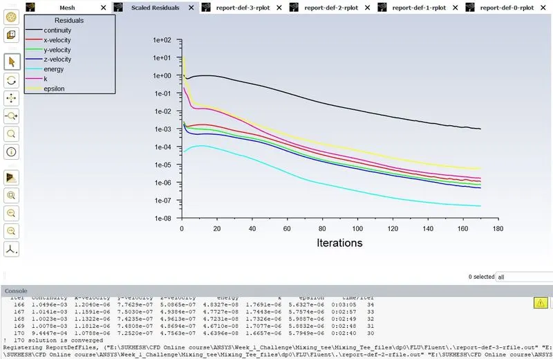
• Residual plot

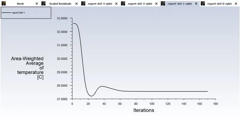
• Area weighted average of temprature at outlet for each iteration

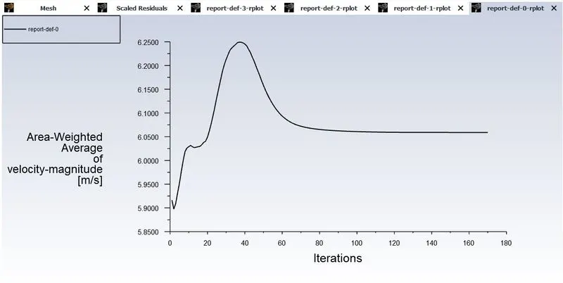
• Area weighted average of velocity at outlet for each iteration

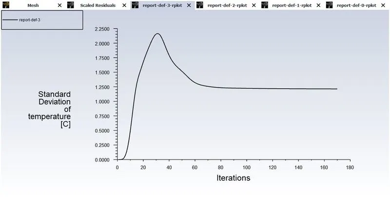
• Standard deviation of temprature at outlet for each iteration

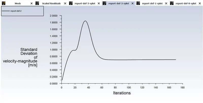
• Standard deviation of velocity at outlet for each iteration

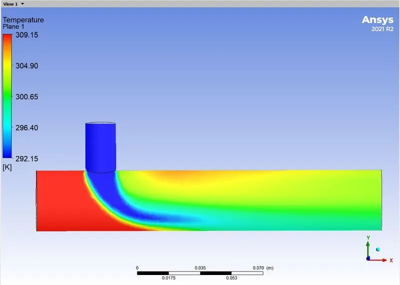
• Temperature contour

• Velocity contour

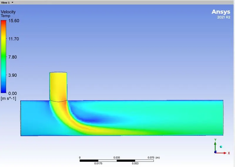
Long mixing-Tee with momentum ratio = 2

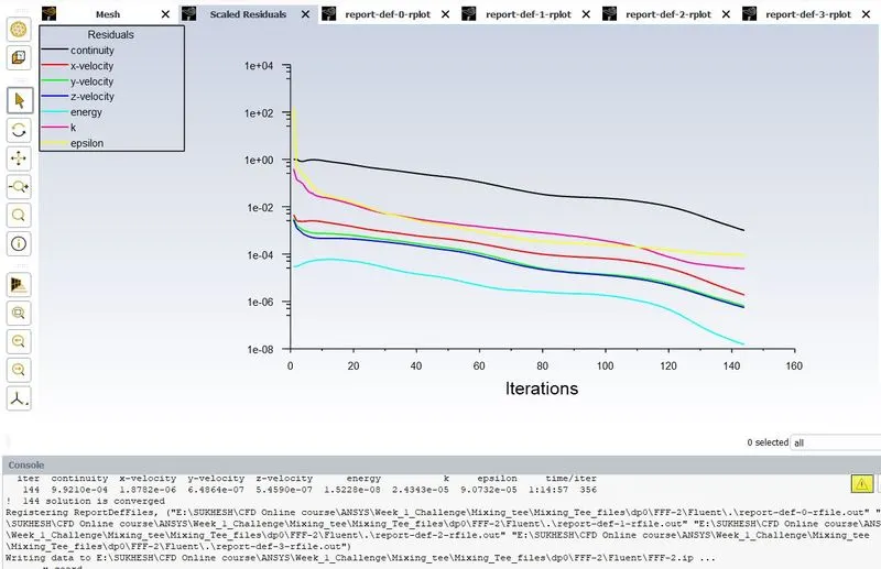
• Residual plot

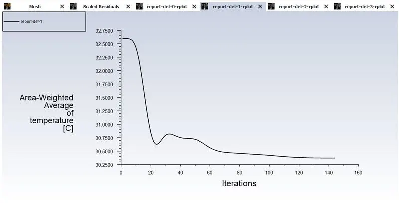
• Area weighted average of temprature at outlet for each iteration

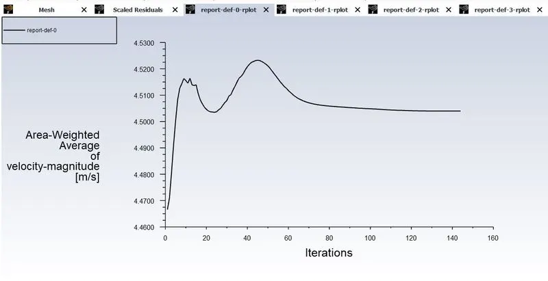
• Area weighted average of velocity at outlet for each iteration

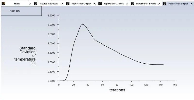
• Standard deviation of temperature at outlet for each iteration

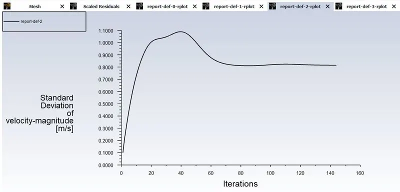
• Standard deviation of velocity at outlet for each iteration

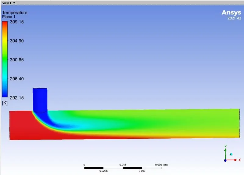
• Temperature contour

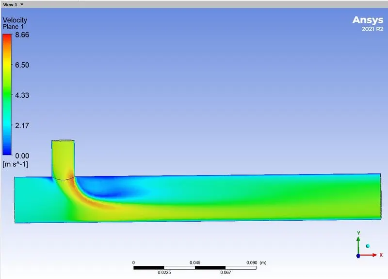
• Velocity contour

Long mixing-Tee with momentum ratio = 4

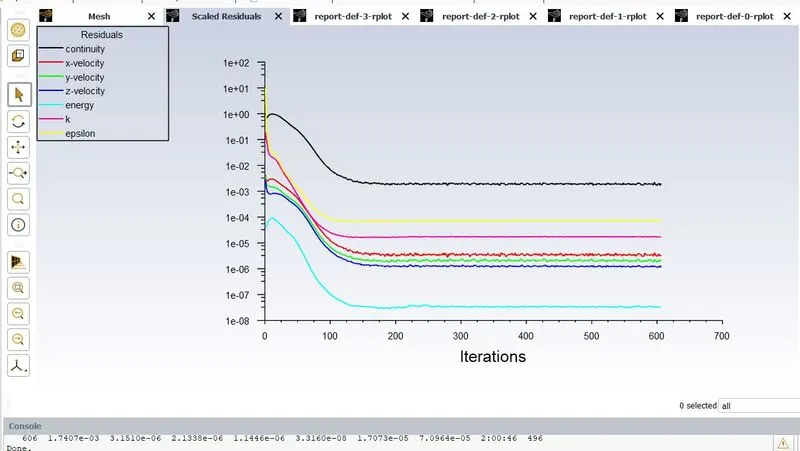
• Residual plot

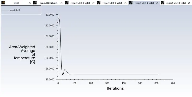
• Area weighted average of temprature at outlet for each iteration

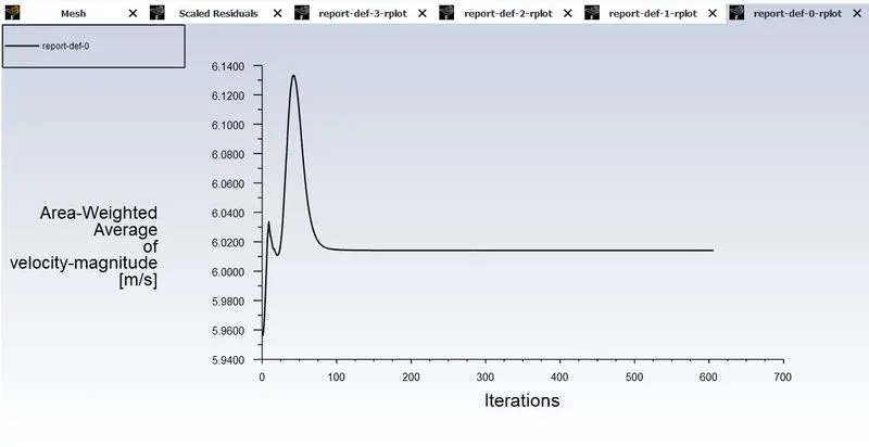
• Area weighted average of velocity at outlet for each iteration

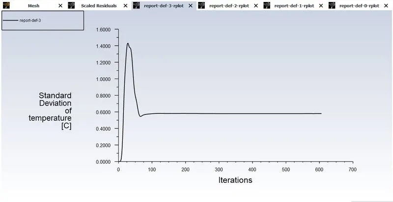
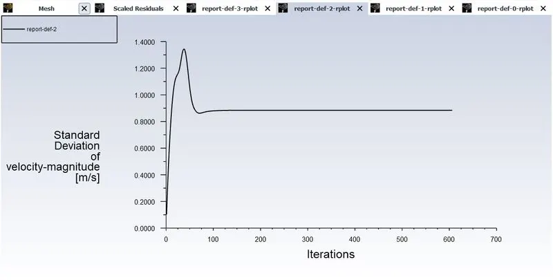
• Standard deviation of temperature at outlet for each iteration

• Standard deviation of velocity at outlet for each iteration

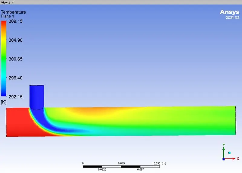
• Temperature contour

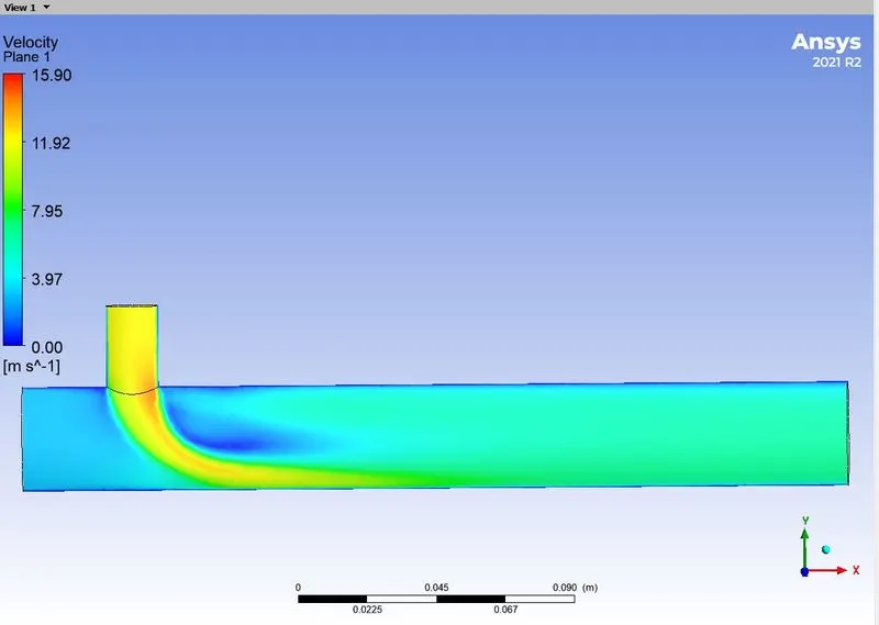
• Velocity contour

Comparison of the two cases

Cases	Cell count	Average outlet temperature (K)	Number of iterations for convergence
Case 1 Short-T (momentum ratio=2)	564818	303.50	138
Case 1 Short-T (momentum ratio=4)	564818	300.82	170
Case 2 long-T (momentum ratio=2)	755032	303.58	144
Case 2 long-T (momentum ratio=4)	755032	300.65	606

CONCLUSION

• The outlet temperature of the combined air shows that the mixing efficiency increases with increasing momentum ratio. As the momentum ratio is increased the cold inlet velocity increases which inturn helps in better mixing of the fluids in the pipe.
• Temperature contour of short-T and Long-T with momentum ratio = 2 and momentum ratio = 4 shows that as length of the mixing-T increases the mixing effectivenss increases. Hence Long-T has uniform temprature drop in the outlet. This can be evidently concluded by looking into the standard deviation of temperature line plots.