Week 1- Mixing Tee

Aim

Performing Simulation of a 'mixing tee' apparatus requiring mixing of fluids(air) at different temp of 19 and 36 celcius with a momentum ratio as mentioned below:-

1. Case 1
   • Short mixing tee with a hot inlet velocity of 3m/s.
   • Momentum ratio of 2, 4.
2. Case 2
   • Long mixing tee with a hot inlet velocity of 3m/s.
   • Momentum ratio of 2, 4.

Momentum ratio = velocity at cold inlet / velocity at hot inlet

After simulation, discuss on the various results we get for different parameters like choosing k-epsilon and k-omega SST model for the first case.

Introduction

Turbulent mixing of fluid of different temperature in T-junction geometries became of significant importance in the field of nuclear reactor safety, since it can lead to highly transient temperature fluctuations at the adjacent pipe walls, cyclic thermal stresses in the pipe walls and consequently to thermal fatigue and failure of the pipeline.

The choosing of right model is very important,based upon the physics applied in our application. The decesion of choosing Steady State model or turbulent flow model (choosing k-epsilon and k-omega) will highly decide our results.

Theory

The process fluesnt fluid flow will be done in following these 5 steps:-

1) Geometry - The geometry of the model will be formed where the actual flow will flow/interfere

2)Mesh - The meshing of the volume is done whoose parameters are set by default with help of 'Boundary Box'

3)Setup - The initial and boundary conditions or parameters and the model choosen are given to the model.

4) Solutions - Based on conditions and requirements the result is calculated with the help of model choosen

5) Results - The final results are appeared here from where the investigation of simulation is done.

Solving & Modelling Approach

I have soved through the stages mentioned above with the help of videos shown and guidance of the technical staff.

0) Download the step file of model available to us.

1) Geometry - The geometry of the model will be formed where the actual flow will flow/interfere.

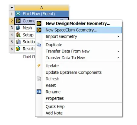
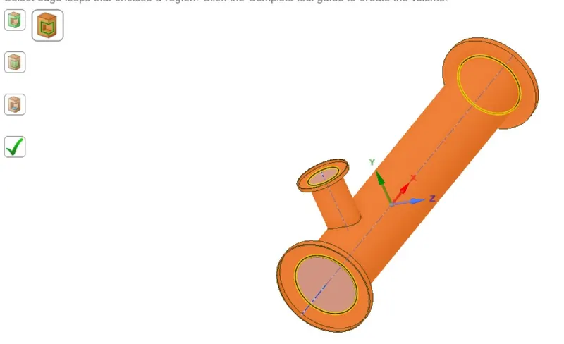
1.1) Select only the region where the fluid interfere with help of VOLUME EXTRACT feature.

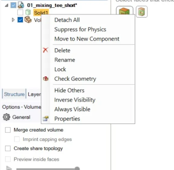
1.2) 'Supress for physics' and hide' the solid part.

1.3) Close the window and open the Mesh window from workbench.

Pre-processing and solver setting

2)Mesh - The meshing of the volume is done whoose parameters are set by default with help of 'Boundary Box'

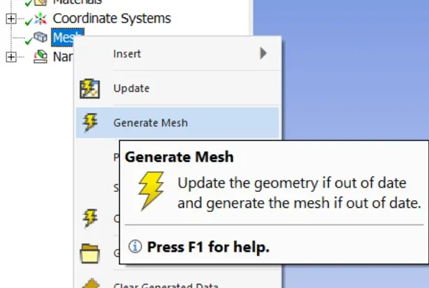
2.1) Generate meshing was performed to give the meshed product.

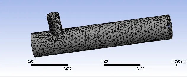
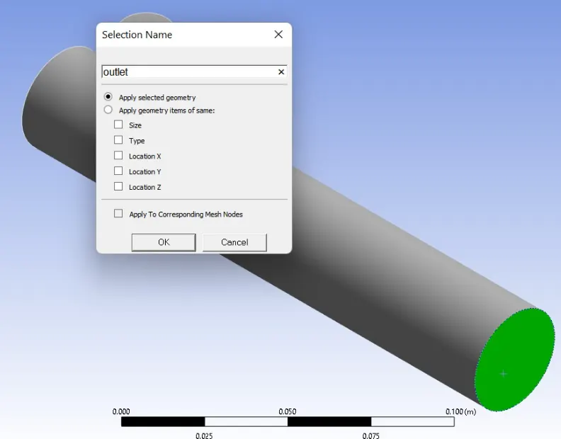
2.2) Give names to the faces as:-

1. Inlet x

2. Inlet y

3. Outlet

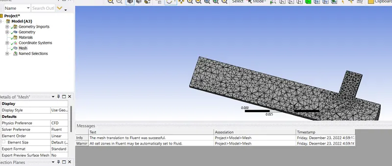
2.3) Investigate the mesh produced with help of SECTIONAL VIEW feature

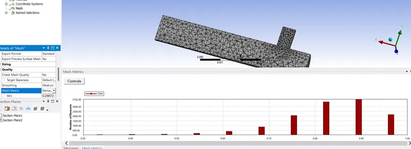
2.4) Check the quality of mesh to be more than 5%

2.5) Then close the window + update mesh + open Setup

3)Setup - The initial and boundary conditions or parameters and the model choosen are given to the model.

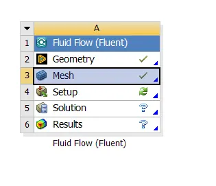
3.1) Check the status whic should say 'done' and then switch to graphics

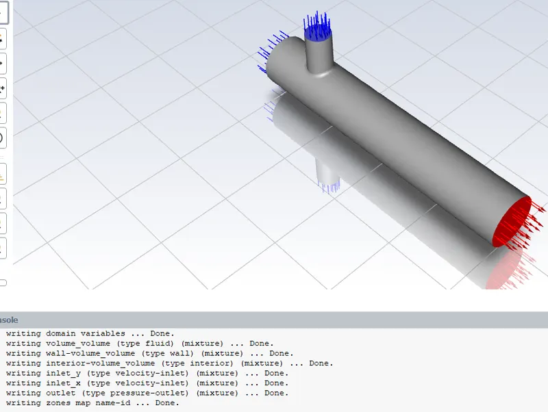
3.2) Set up the physics as shown below

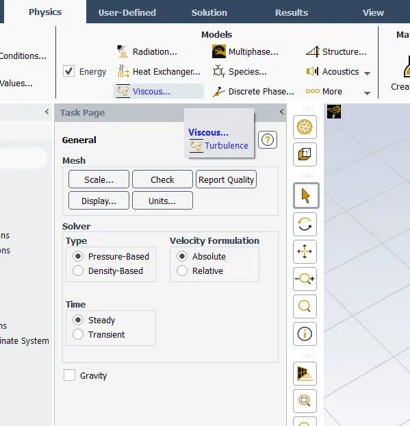
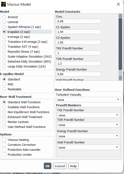
3.3) At viscious give the both k-epsilon and k-omega 1-by-1

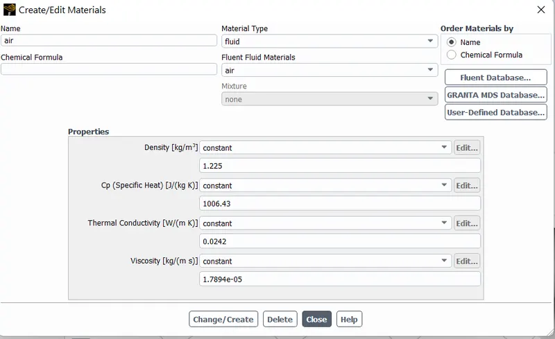
3.4) Check the material to be 'Air' if not then use the fluid DB

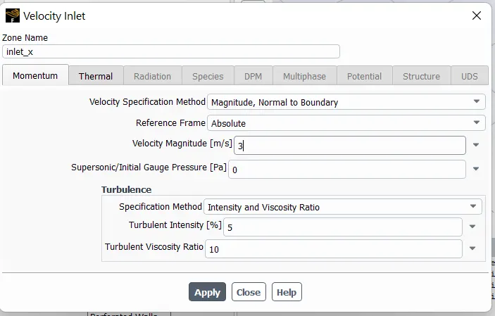
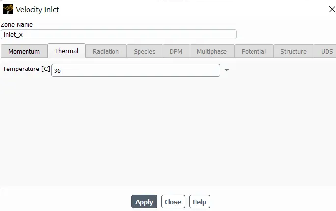
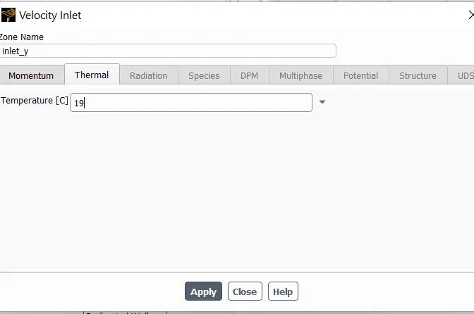
3.5) It's time to assign Boundary Conditions (BC) and give :-

1. Hot inlet velocity = 3m/s.

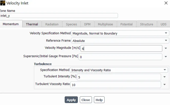
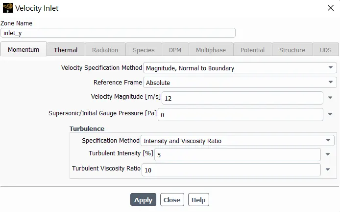
2. Cold inlet velocity = 6m/s & 12m/s for 2nd case.

3. Hot Inlet temp = 36 C

4. Cold Inlet temp = 19 C

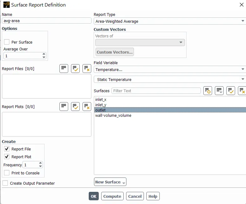
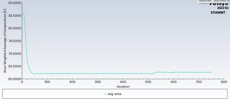
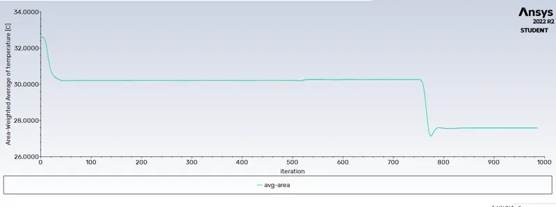
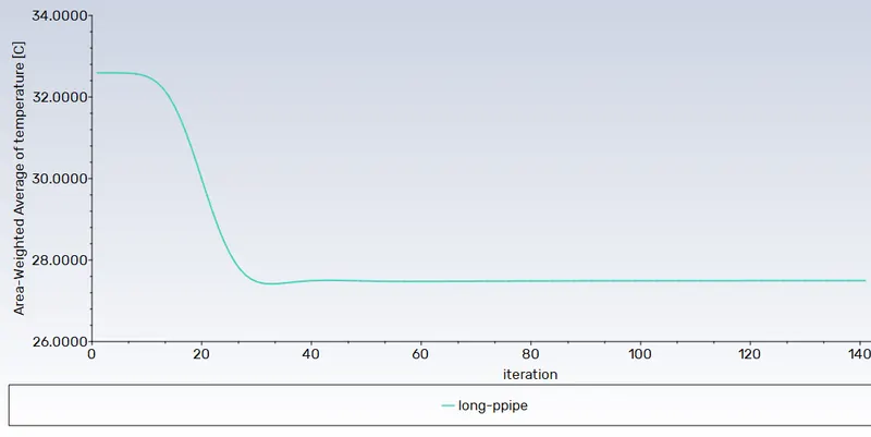
3.6) For result reports define the for new srface area with 'Area-Weighted Temp' parameter as variable.

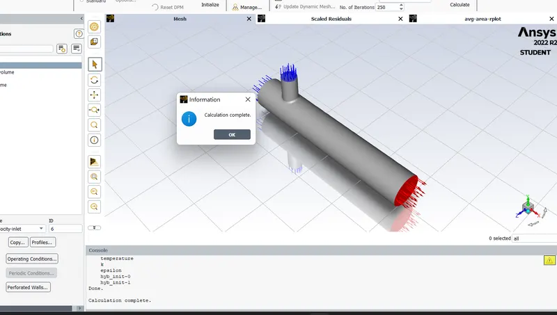
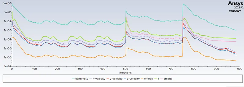
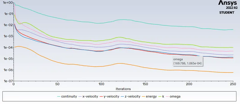
3.7) Give 250 no. of iterations and calculate the result.

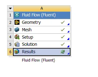
3.8 ) After the graphical results appears, close the window and open the 'Result' from WorkBench

4) Solutions - Based on conditions and requirements the result is calculated with the help of model choosen.

This step is done and completed by the computer itself based on the calculated results of Setup.

5) Results - The final results are appeared here from where the investigation of simulation is done.

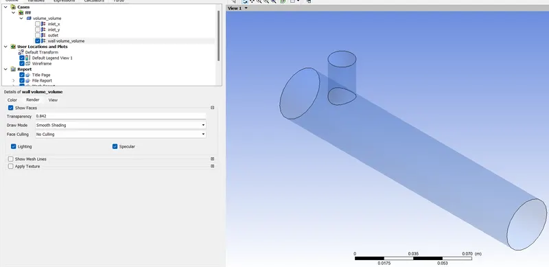
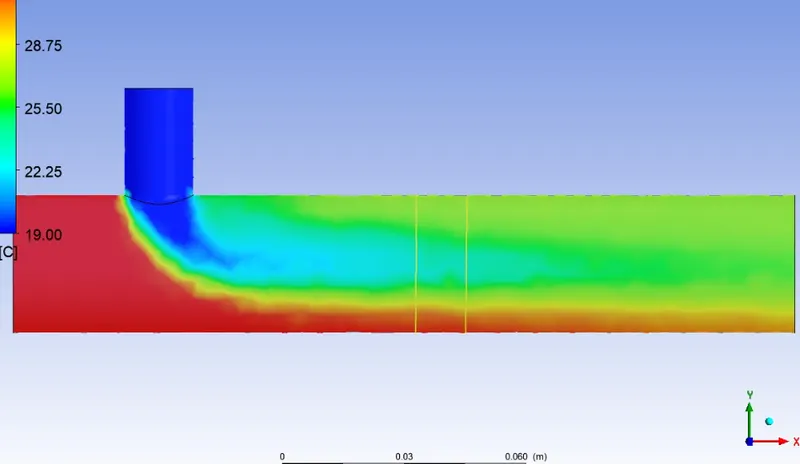
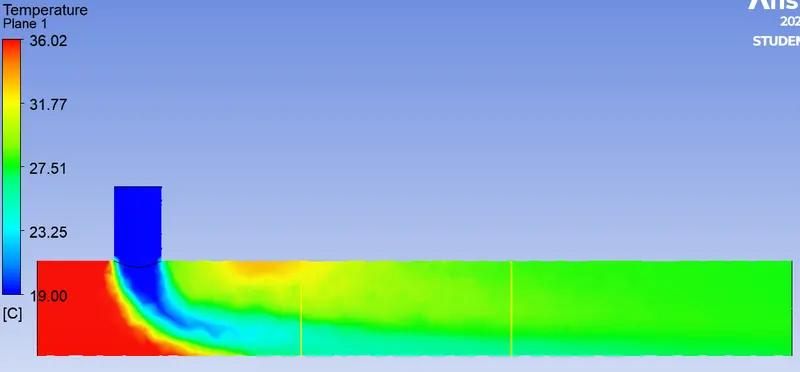
5.1) The post-processing begins, from render increase the transpirancy of pipe walls.

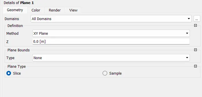
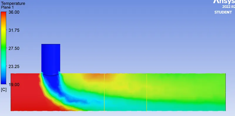
5.2) Insert a plane in XY where the results are simulated and shown

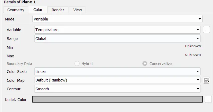
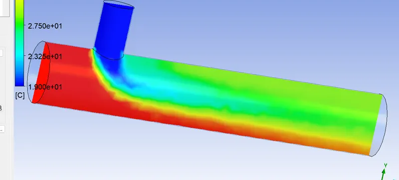
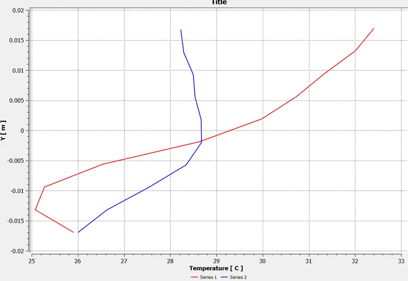
5.3) Projects 2 lines on it by giving it starting and end points

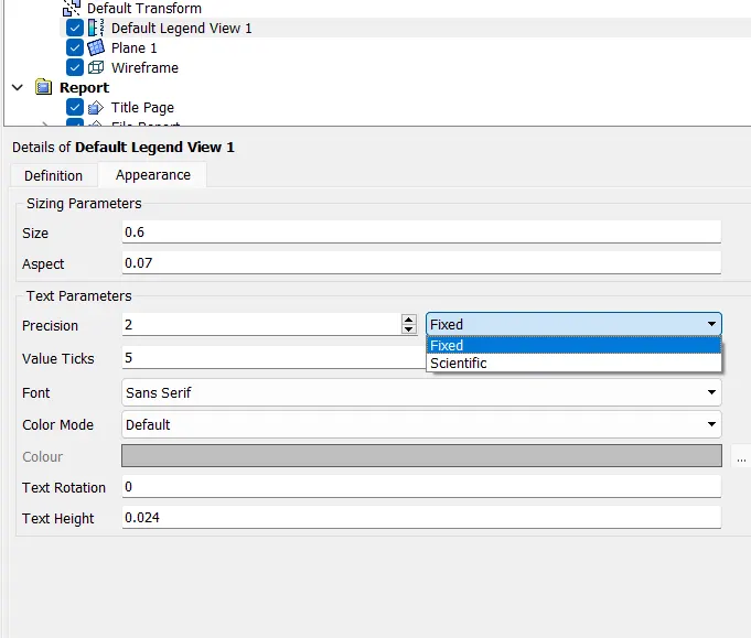
5.4) Simplify the Legend-view from 'DEFAULT LEGEND VIEW' by changing it to 'FIXED'

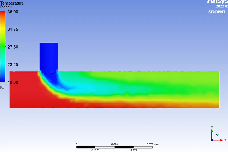
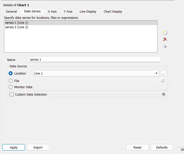
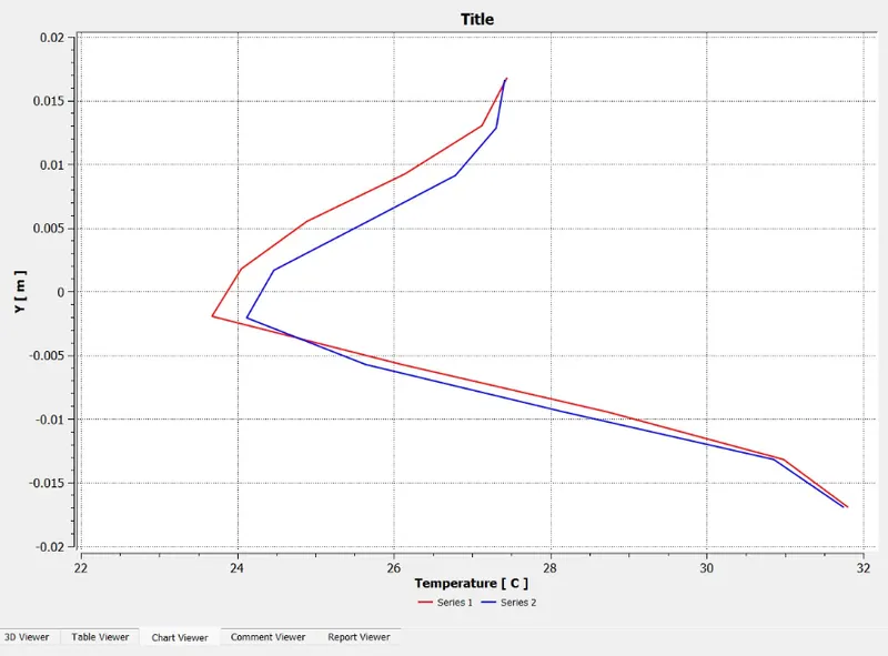
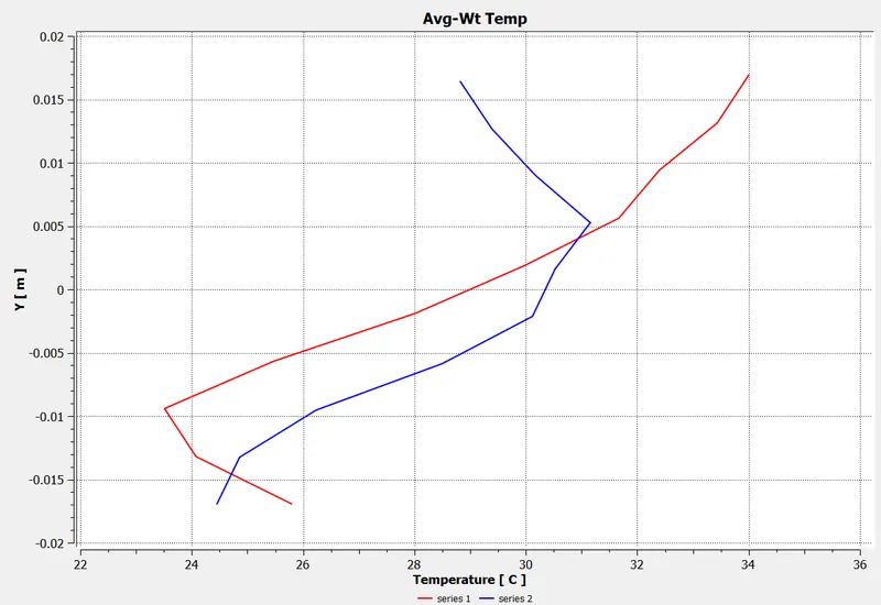
5.5) Insert a chart for analysis and comparision

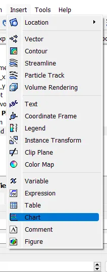
5.6) Insert lines

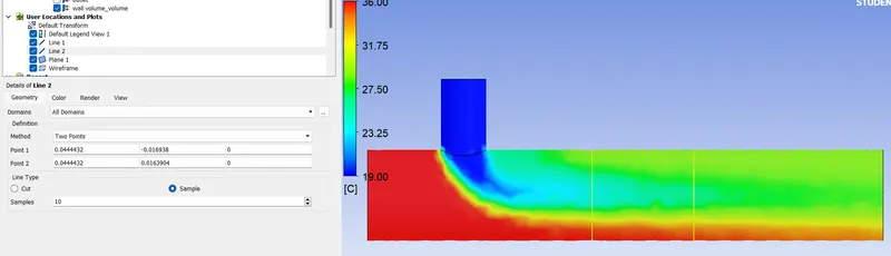
5.7) Assign Series 1 & 2 as line 1 & 2 respectively.

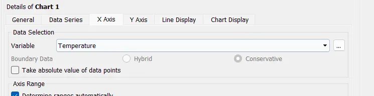
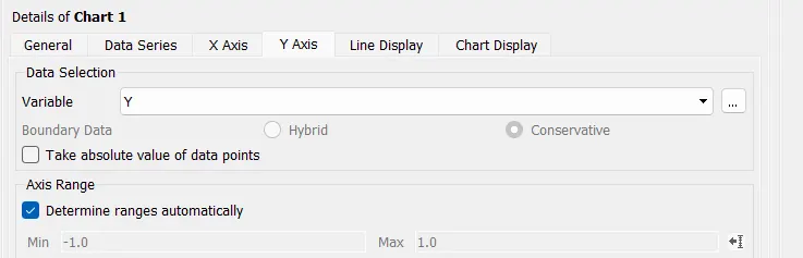
5.8) Assingn the parameters to the axes of the chart.

Results

The 3D view and chart is given below for each case obtained:-

1) Short Pipe + M.R.(2) + k-epsilon Momentum ratio(M.R.) = velocity at cold inlet / velocity at hot inlet

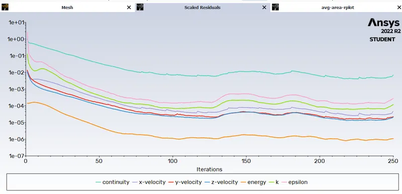
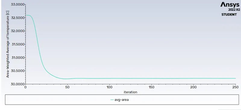
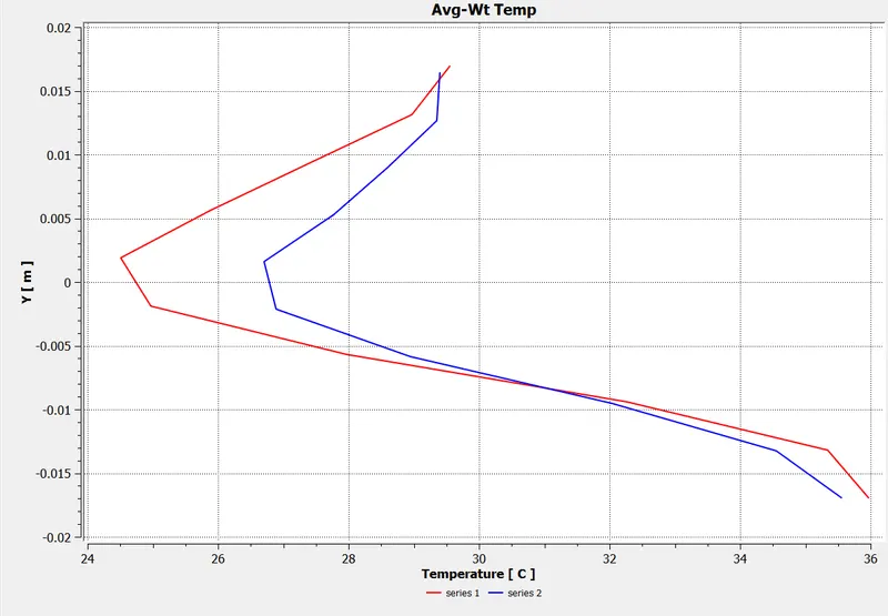
2) Short Pipe + M.R.(2) + k-omega

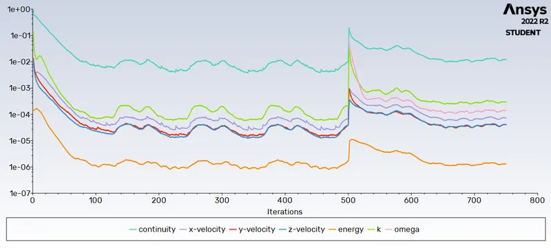
3) Short Pipe + M.R.(4) + k-omega

4) Large Pipe + M.R(2) + k-omega

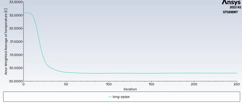
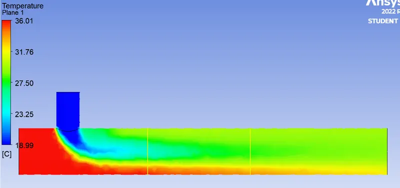
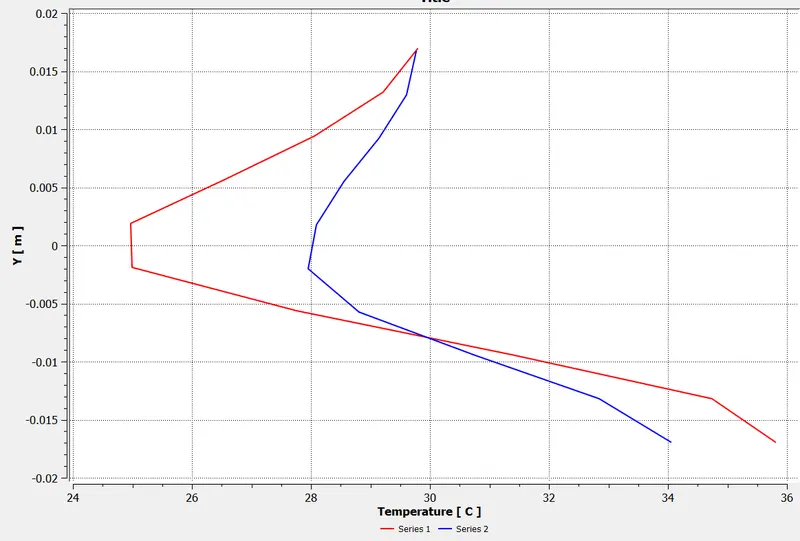
5) Large Pipe + M.R(4) + k-omega

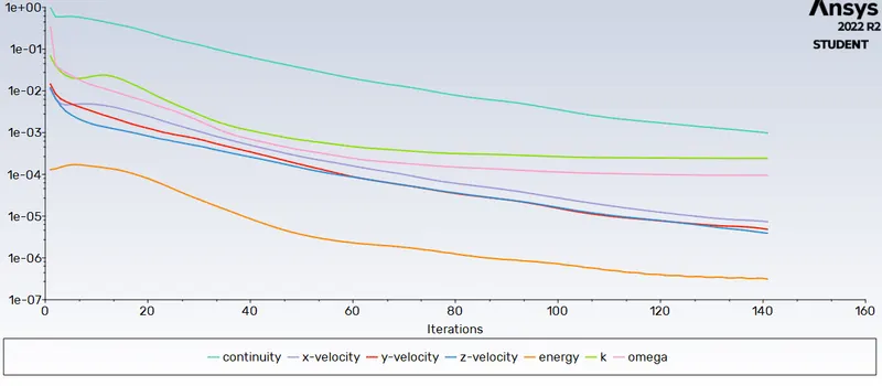
	Short Pipe + M.R.(4) + k-omega	Large Pipe + M.R(2) + k-omega
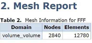
Cell count	12780 elements	15727 elements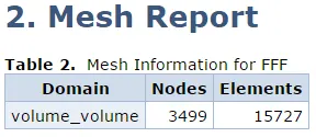
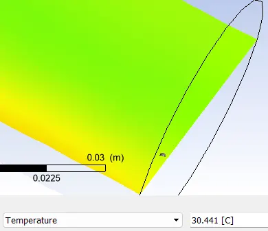
Average outlet temperature	31.8 C	30.4 C
Number of iterations for convergence	60 iterations	60 iterations

Conclusion

From this simulation we can conclude that:-

1. The smaller the mesh element size the finer result is and longer it would take for processing.

2. The outlet temperature is almost same for small and larger pipe for high M.R, but for smaller M.R the outlet temp of long pipe will be lower as compared to the short pipe.

3. From the results it can be said that K-omega is better for near wall analysis while K-epsilon gives better result for far point from the walls.

The best system for CFD would the one which used K-omega near walls and K-epsilon for the bulk.

4. Both long and short pipe takes almost same time to converge.