Week 1- Mixing Tee

Aim: Simulation of a mixing Tee to evaluate effectiveness when hot inlet temperature is 36 deg C & the Cold inlet is at 19 deg C for a short and long mixing tube.

Objective –

1. To extract fluid volume from the geometry and mesh it in pre-processing.
2. To solve the model with best solver in Ansys solver.
3. To generate contour and line plots and analyse it in postprocessor.

Introduction –

Computational fluid dynamics is a branch of fluid mechanics, which uses mathematics, physics and computational software to visualize how fluid flows and affects its medium and its neighbours. In CFD mostly computers are used to predict the fluid flow phenomena based on some governing equations like conservation of momentum – Navier stokes equation, conservation of energy etc. In this study we are going to simulate the effect of fluid using Ansys fluent software. Ansys fluent is a very important tool in CAE domain, which allows you to perform all the three major steps of any simulation pre-processing, solving and post-processing. Ansys fluent facilitates for modelling flow, turbulence, heat transfer and chemical reactions.

Mixing tee is a device which uses specifically engineered internal geometry to mix two fluid streams into one steam, efficiently. In this study we are going to find effectiveness of mixing tee. Hot air and cold air are going to be mixed in mixing tee. They will have different velocities. We will use two different mixing tee distinguished with length and analyse the effect of length on mixing.

Procedure -

There are three major steps to perform any type of simulation as follows pre-processor – it includes geometry clean up and generate best quality mesh. Solving includes applying boundary conditions, initialize and convergence. Last step is post processor which includes generate plots, contours, vectors to analyse results. In this study we are going to follow all three steps to find out effectiveness of mixing tee. The following steps to be followed –

1. Open new project, by clicking on Fluid flow (Fluent) in Ansys workbench.

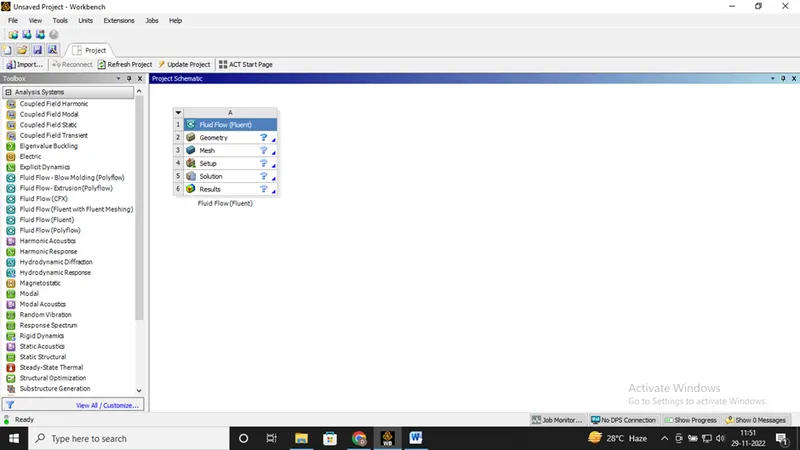2. Now click on geometry to import mixing tee model. It will redirect to Space claim.

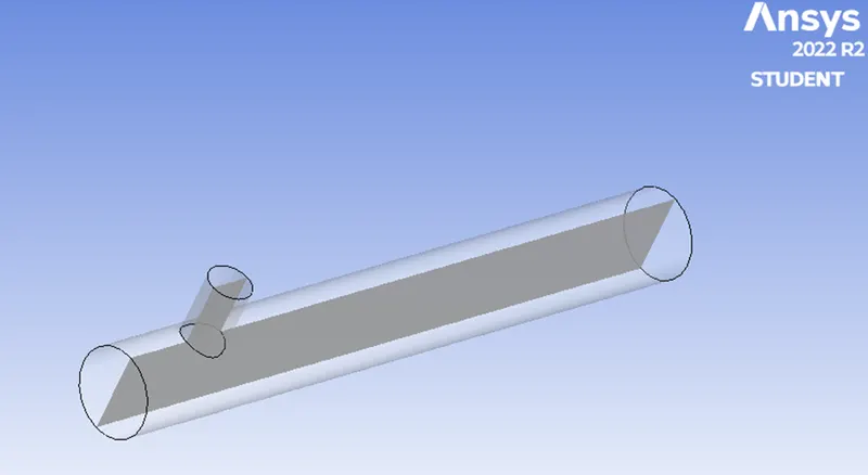
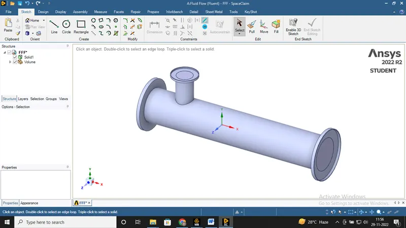3. We are to analyse the mixing of two fluids, so there is role of parts other than two pipes. To supress that we need to extract volume of tee. Go to prepare menu and click on volume extract. Switch to edge selection and select three outer edges and click on green check button.

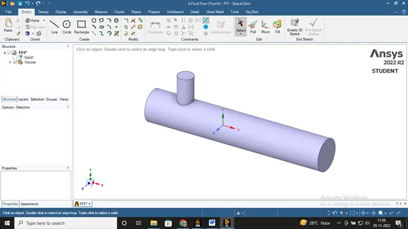
4. Hide solid by unchecking it from structure menu to see volume, which we have extracted. Supress solid by clicking on option supress for physics.
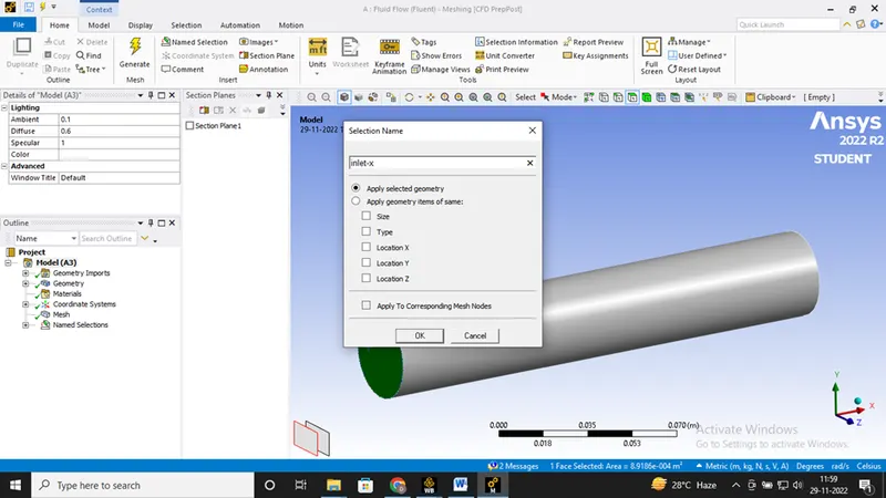
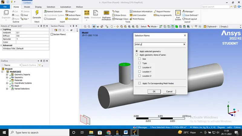
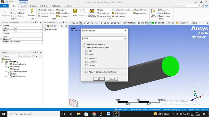
5. Exit from Space claim and click on mesh to open mesh menu. Select outer face and press right click of mouse, it will open a menu. Click on option create named selection and write suitable name for face. Repeat for other faces.

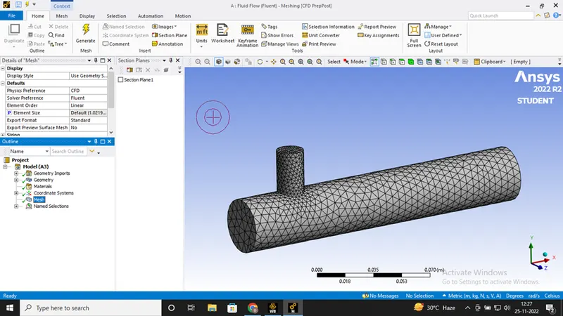
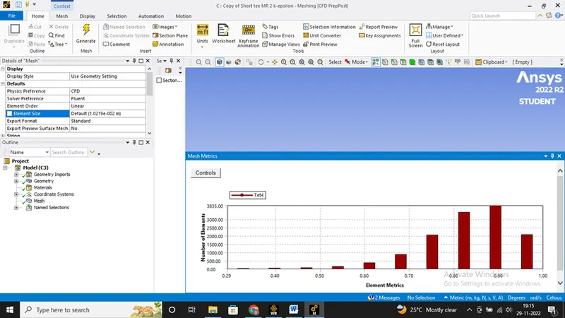
6. Now click on mesh option and choose generate mesh. It will generate mesh according to some predefined criteria. Element size can be selected but it is going to affect simulation time. Select the option element quality to see, how many elements are defying quality. Quality is measured on the scale of 0 to 1. In our graph most of the elements are near to 1 so we can say it is good quality.

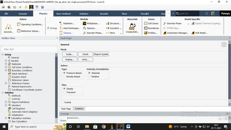
7. Exit mesh and open setup. First, Check mesh, it is throwing no error then only we can proceed further. We are going to do pressure based steady state simulation, so choose these options on task page.

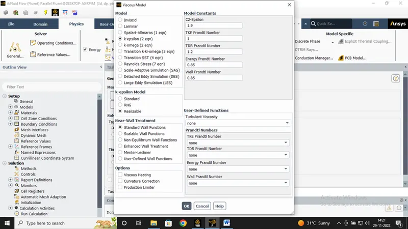
8. Go to physics menu and select viscous model. It will open a menu, choose realizable k-epsilon model and close it.

9. Click on material and choose air as working fluid. Check working fluid by clicking on cell zone conditions option, if it is air then proceed.
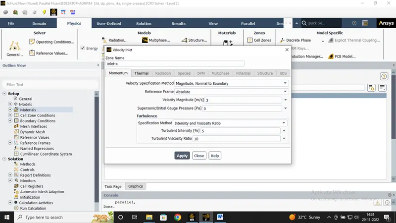
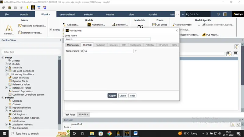
10. Now go to boundaries option to set boundary conditions. Select inlet_x and click on option edit. It will open a menu, where all the parameter can be set whether it is thermal, radiation, momentum etc. Put the value of velocity as 3m/s and go to thermal parameter to set temperature as 36⁰ C, for hot fluid. Repeat the same procedure for cold fluid coming with velocity 6 m/s and temperature 19⁰ C.

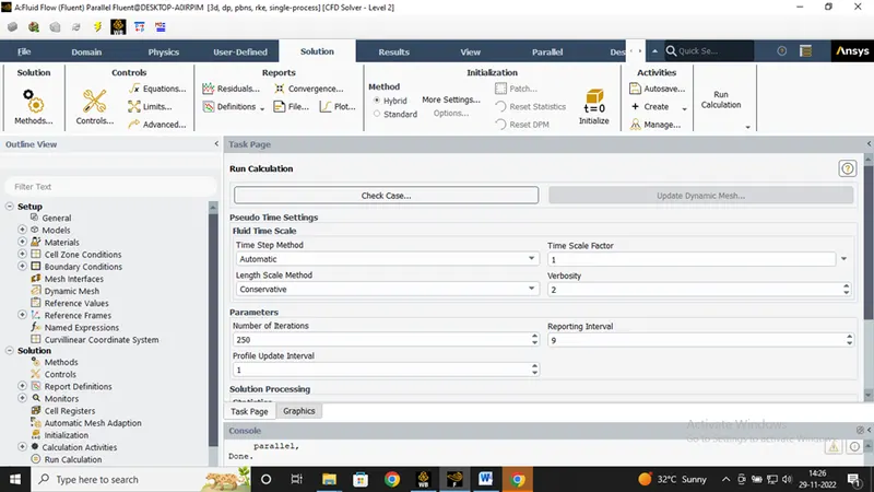
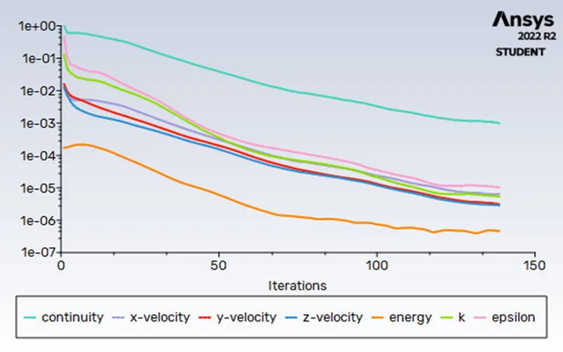
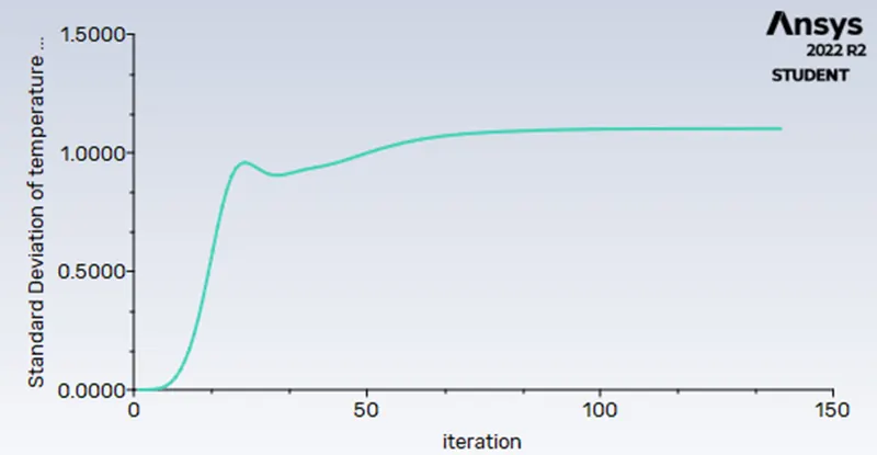
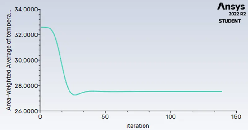
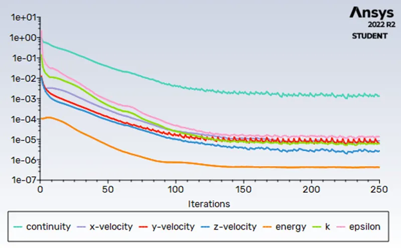
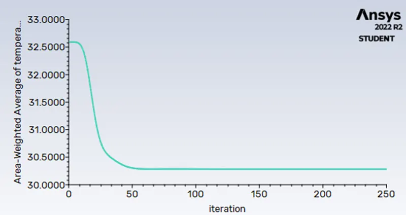
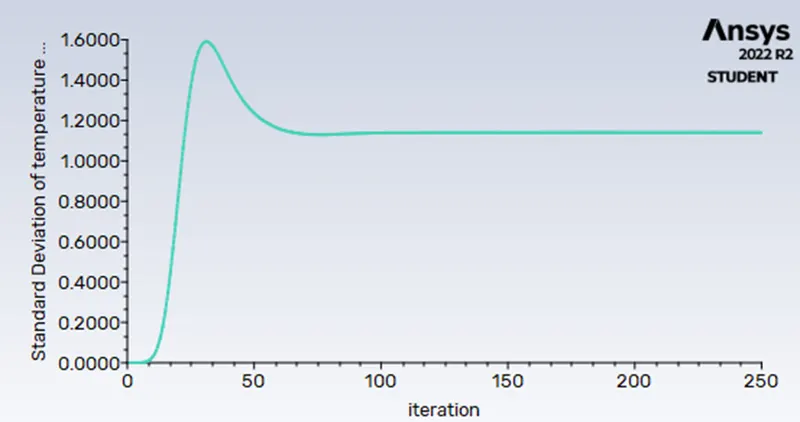
11. We want to generate temperature report of outlet and we want standard deviation of temperature also. Go to solutions tab and select definition and select area weighted average. In the opened menu select temperature as field variable. Similarly select standard deviation in definitions menu. Now click on initialization to calculate approximate values of velocity and pressure. Change the number of iterations to 250 and click on calculate. If solution is not converged, then iterations can be increased.

12. Exit setup and double click on result to open CFD post. Check boxes to see walls and other parts. Click on walls and go to render set transparency of 0.4 to inside of wall. Colour can also be changed to white for clear visibility. Now insert a XY plane in wall by clicking on plane in location option of insert.

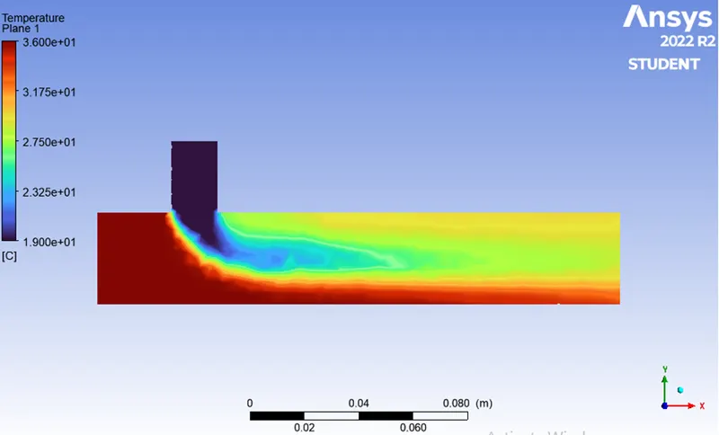
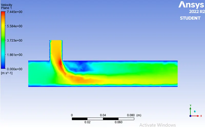
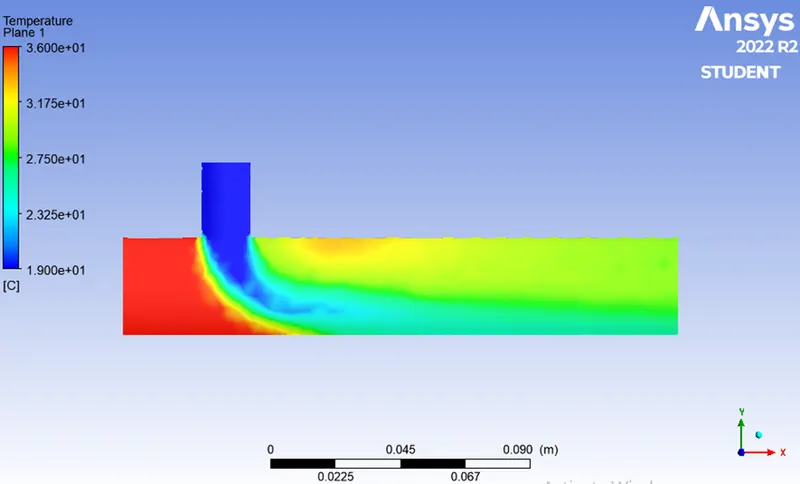
13. Go to colour of plane and change it by variable choose option temperature. Similarly, velocity contours can be created by just changing variable as velocity.

Results –

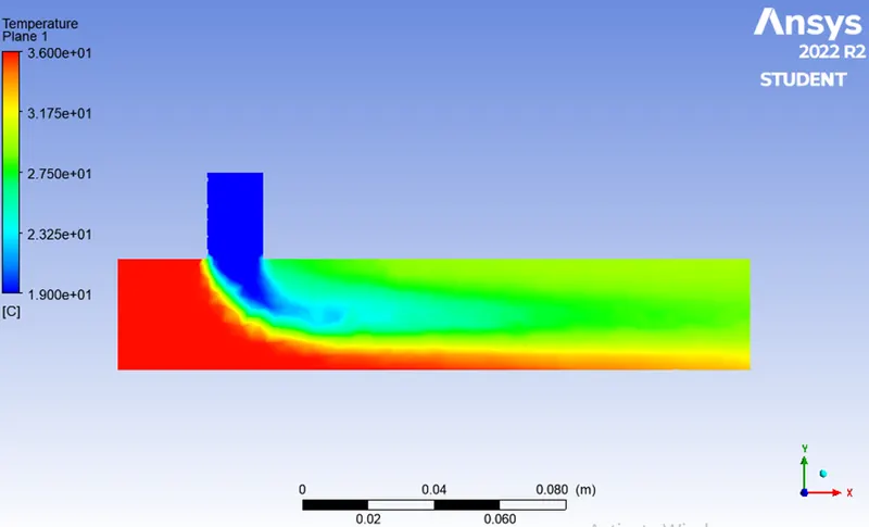
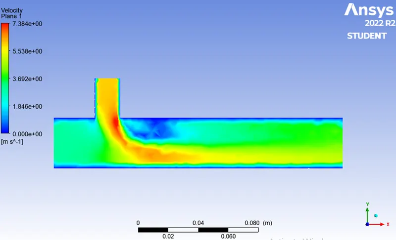
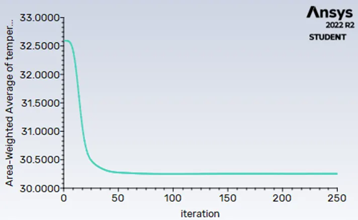
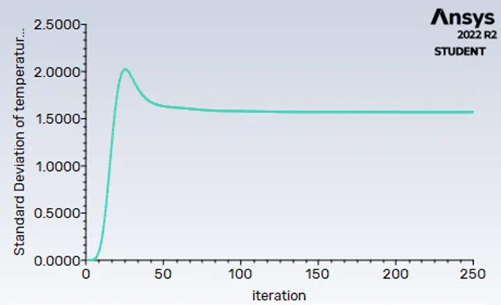
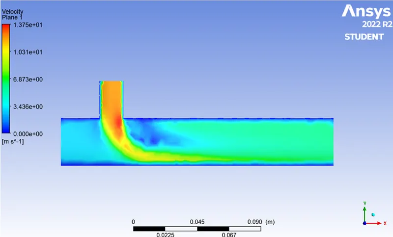
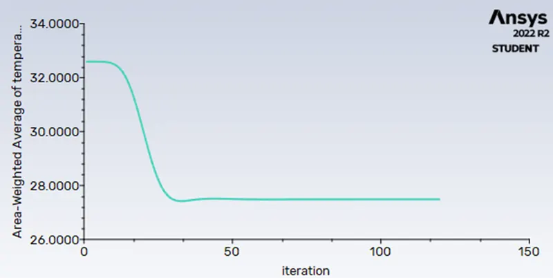
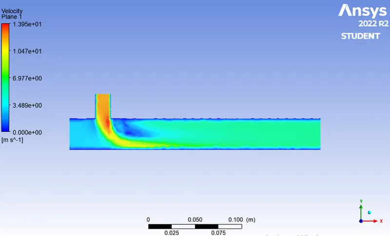
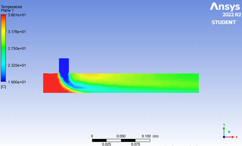
Case 1 – In this short mixing tee is used, which was mixing two fluid with temperature 36C and 19C. Velocity of hot fluid was 3m/s and cold fluid was 6m/s. we used two different turbulent solvers for it first was realized k-epsilon and second was k-omega SST.

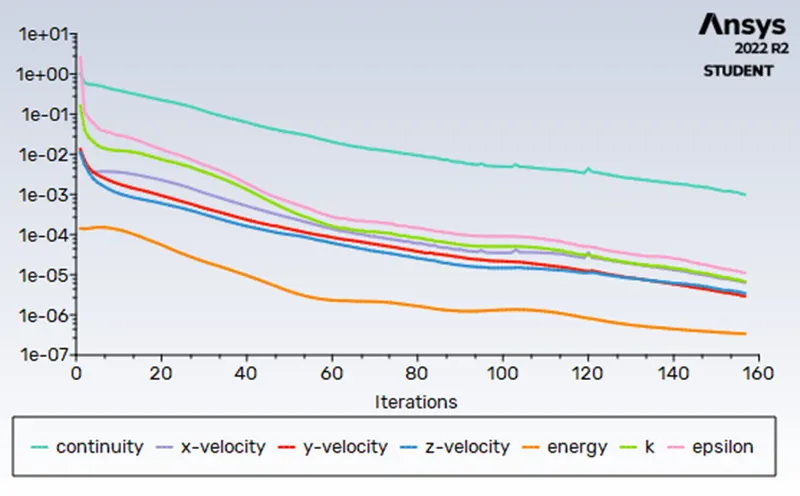
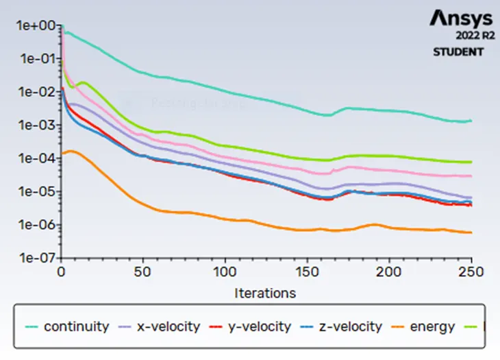
In this case k-epsilon is giving better results because solution was converged after few iterations, whereas after using k-omega model solution was not converged. K-omega is preferred in studying fluid behaviour near wall, but here it is not the case. So, k-epsilon model is recommended to study of fluid far from wall i.e. flow region, in further cases.

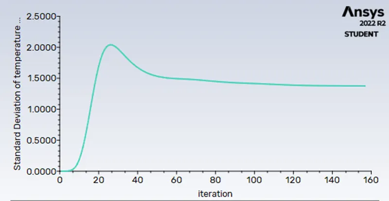
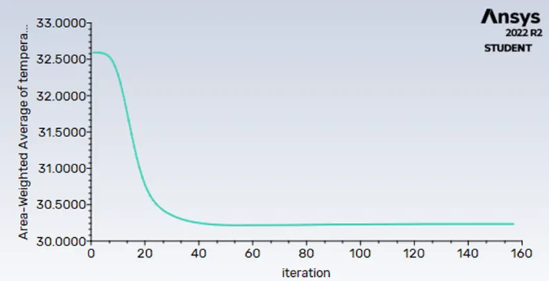
Plot and contours from k-epsilon model (MR 2/short Tee)

Plot and contours from k-omega model (MR 2/short Tee)

Plot and contours from k-epsilon model (MR 4/short Tee)

Case II:

Plot and contours from k-epsilon model (MR 2/Long Tee)

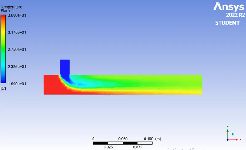
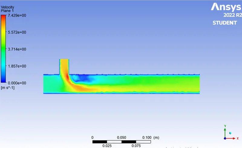
Plot and contours from k-epsilon model (MR 4/Long Tee)

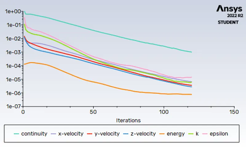
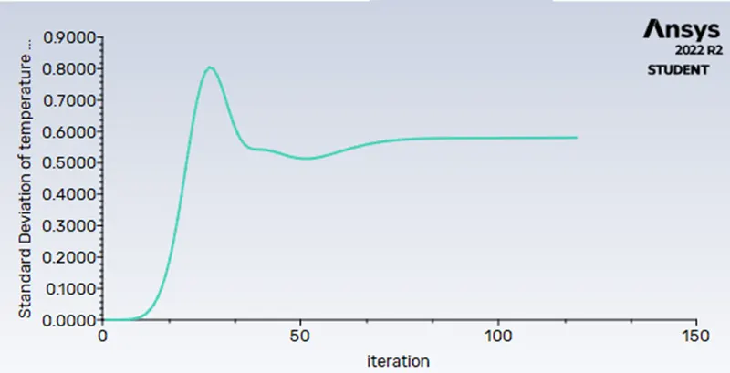
	k-ε model		k-ω model	k-ε model
Particulars	Short Tee		Short Tee	Long Tee
	MR 2	MR 4	MR 2	MR 2	MR 4
Cell count	12742	12742	12742	15663	15663
Avg. Temperature outlet (C)	30.22	27.5	30.24	30.26	27.46
No. of iterations	160	140	250	150	120
Standard deviation of temperature	1.36	1.09	1.55	1.6	0.6

Table: Partculars for different case studies

CONCLUSION:

Case 1: On comparing both the models of k-ε and k-ω for short mixing Tee with MR 2, the results observed was nearly the same. But, No. of iterations taken to converge is less for Realisable K-epsilon model than K-omega SST model.

The standard deviation of k-epsilon model is less than k-omega model which shows the better mixing efficiency in k-epsilon model.

Hence, based on the above observations the K-epsilon turbulence model is predicting the results accurately in less no. of iterations. So we can use realisable k-epsilon model for further studies in case of long Tee mixing.

Case 2: From the comparison of short and long Tee simulation results, it was observed that irrespective of length of the mixing Tee, the average outlet temperature on both cases are quite same.

As momentum ratio increases, the velocity of cold inlet fluid increases and due to high relative velocity between the fluid it experiences higher turbulence and therefore the outlet fluid temperature decreases.

For momentum ratio 2, the average outlet fluid temperature is 30.26⁰ C whereas for momentum ratio 4 the average outlet fluid temperature is 27.46⁰ C. From these we can say that there will be a drop in temperature if momentum ratio increases.

In order to obtain better mixing the velocity of cold fluid is important. By increasing the cold fluid velocity the outlet temperature gets reduced. Higher the momentum ratio, higher will be the mixing efficiency of Tee joint. Increasing the length of the pipe doesn’t serve the purpose of mixing efficiently. So, it is efficient to use short pipe.

Grid independent study

For studying the grid independence, the short Tee with MR 2 has been considered. The following three mesh grid sizes have been undertaken for the study.

Sl no.	Mesh size (mm)	No. of elements	Avg. outlet temperature (C)
Case I	0.01	12742	30.22
Case II	0.007	12846	30.24
Case III	0.005	14113	30.25

From above table we can say that our mesh is independent that means there is no large changes in outlet temperature by increasing the number of elements. Hence, we can prefer less number of mesh for the simulations.