Week 4.1 - Solving second order ODEs

Aim-Solve a second order ordinary differential equation using Matlab code.

Objectives-

1. Write a Matlab code to solve ODE demonstrating the motion of a simple pendulum.
2. Plotting the graphs of the displacement and the velocity with time.
3. Create an animation of the motion of the simple pendulum.

In mathematics, an ordinary differential equation (ODE) is a differential equation containing one or more functions of one independent variable and the derivatives of those functions. The term ordinary is used in contrast with the term partial differential equations which may be with respect to more than one independent variable.

The way the pendulum moves depends on Newton’s second law. When this law is written down, we get a second order Ordinary Differential Equation that describes the position of the "ball" w.r.t time. In Engineering, ODE is used to describe the transient behaviour of a system. A simple example is a pendulum.

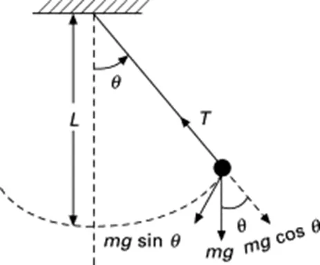
The motion of a simple pendulum can be depicted by a second order ordinary differential equation. The governing equation is shown below-

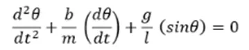
In the above equation,

g = gravity in m/s2,

L = length of the pendulum in m,

m = mass of the ball in kg,

b=damping coefficient.

Matlab code-

close all

clear all

clc

b=0.05;

g=9.81;

l=1;

m=1;

%initial condition

theta_0=[0;3];

%time points

t_span=linspace(0,20,500);

%solve ODE

[t, results]=ode45(@(t,theta) ode_func(t, theta, b,g,l,m),t_span,theta_0);

figure(1)

plot(t,results(:,1))

hold on

plot(t,results(:,2))

ylabel('plot')

xlabel('time')

legend("Angular displacement","Angular velocity")

% Writing a for loop to make the animation

ct = 1;

for i = 1:length(results(:,1))

x0 = 0;

y0 = 0;

x1 = l*sin(results(i,1));

y1 = -l*cos(results(i,1));

% Plotting the animation

figure(2)

plot([-1 1],[0 0],'linewidth',5)

hold on

plot([x0 x1],[y0 y1],'linewidth',3)

hold on

plot(x1,y1,'o','markersize',20,'markerfacecolor','y')

axis([-2 2 -2 2])

pause(0.03)

M(ct) = getframe(gcf);

ct = ct+1;

hold off

end

% Making a movie/animation

movie(M)

videofile = VideoWriter('pendulum.avi','Uncompressed AVI');

open(videofile)

writeVideo(videofile,M)

close(videofile)

Explanation of the code-

1. At the very beginning, the given initials are assigned in the code.
2. The initial values of displacement and velocity are given by theta_0 in column matrix format.
3. Using linspace command the time period (0-20) is set for pendulum motion.
4. Create a separate anonymous function of ode_func and then use ode_45 command to solve the given differential equation.
5. Plot the graphs of displacement and velocity with time by using plot command.
6. To create the animation of the pendulum for loop is used. Within for loop the initial and final positions are defined. The counter command is used to make the value changes in each for loop. Marker command is used for making bob of the pendulum
7. The animation is then plotted and converted to a movie using the video writer command.

Results-

Graph-Displacement vs. Time and Velocity vs. Time

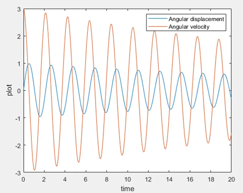
The graph shows the Displacement and Angular velocity in blue and red colour respectively, which are decreasing with respect to the increased time. This happens due to the introduction of Damper, which absorbs the vibrations to make the body in equilibrium position.

The link for the animation video uploaded in YouTube is given below-

https://youtu.be/29ImSmC4Fe0

Conclusion-

1. Using Matlab code, we are able to solve the equation of a second order ordinary differential equation.
2. We are able to plot the graphs of the displacement and velocity with time demonstrating the oscillating motion of a simple pendulum.
3. An animation of the oscillating motion of a simple pendulum for the given condition is also created.