Week 5 - Genetic Algorithm

Aim- Write a code in MATLAB to optimize the stalagmite function and find the global maxima of the function.

Objectives-

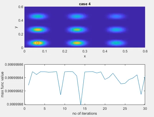
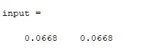
1. Find the global maxima of the given stalagmite function using MATLAB code.

2. Explain the concept of genetic algorithm and also explain the syntax for GA in MATLAB in the report.

3. Make sure that your code gives the same output, even if it is made to run several times.

4. Plot graphs for all 3 studies and for F maximum vs no. of iterations.

Theory-

A genetic algorithm is a search heuristic that is inspired by Charles Darwin’s theory of natural evolution. This algorithm reflects the process of natural selection where the fittest individuals are selected for reproduction in order to produce offspring of the next generation.

There are different phases in the genetic algorithm which have been shown below-

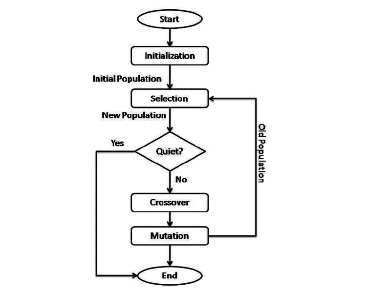
1. Initialization of population-

The process begins with a set of individuals which is called a Population. Each individual is a solution to the problem you want to solve. An individual is characterized by a set of parameters (variables) known as Genes. Genes are joined into a string to form a chromosome (solution). 

2. Fitness function-

The fitness function determines how fit an individual is (the ability of an individual to compete with other individuals). It gives a fitness score to each individual. 

3. Selection-

The goal of selection phase is to select the fittest individuals and let them pass their genes to the next generation. Two pairs of individuals (parents) are selected based on their fitness scores.

4. Reproduction through crossover and mutation-

The generation of Offsprings (new individuals with better fitness) are made through reproduction process. Offsprings are created by exchanging the genes of parents among themselves. Crossover and mutation are the common ways of reproduction.

Flowchart of a genetic algorithm-

Main code-

close all

clear all

clc

 

% Stalagmite function optimization using GA

x=linspace(0,0.6,150);

y=linspace(0,0.6,150);

limit=30;

% create 2D array

[xx yy]=meshgrid(x,y);

for i=1:length(xx)

for j=1:length(yy)

input_vector(1)=xx(i,j);

input_vector(2)=yy(i,j);

f(i,j)=stalagmite_fun(input_vector);

end

end

tic

for i=1:limit

[input,fval(i)]=ga(@stalagmite_fun,2);

x_out(i)=input(1);

y_out(i)=input(2);

end

case_time_1=toc

figure(1)

subplot(2,1,1)

surfc(xx,yy,-f)

xlabel('x')

ylabel('y')

title('case-(unbounded','color','k')

shading interp

hold on;

plot3(x_out,y_out,-fval,'marker','o','markersize',6,'Color','r');

subplot(2,1,2)

plot(-fval);

xlabel('no of iterations')

ylabel('max func value')

 

 

%case 2: inserting bounding box

tic

for i=1:limit

[input,fval(i)]=ga(@stalagmite_fun,2,[],[],[],[],[0;0],[0.6;0.6]);

x_out(i)=input(1);

y_out(i)=input(2);

end

 

 

case_time_2=toc

figure(2);

subplot(2,1,1)

hold on;

surfc(xx,yy,-f)

xlabel('x')

ylabel('y')

title('case 2','color','k')

shading interp

plot3(x_out,y_out,-fval,'marker','o','markersize',6,'Color','r');

subplot(2,1,2)

plot(-fval);

xlabel('no of iterations')

ylabel('max func value')

%case_3

options=optimoptions('ga');

options=optimoptions(options,'populationsize',100)

tic

for i=1:limit

[input,fval(i)]=ga(@stalagmite_fun,2,[],[],[],[],[0;0],[0.6;0.6],[],[],options);

x_out(i)=input(1);

y_out(i)=input(2);

end

case_time_3=toc

figure (3)

subplot(2,1,1)

hold on

surfc(xx,yy,-f)

xlabel('x');

ylabel('y');

title('case 3','color','k')

shading interp

hold on;

plot3(x_out,y_out,-fval,'marker','o','markersize',6,'Color','r');

subplot(2,1,2)

plot(-fval);

xlabel('no of iterations')

ylabel('max func value')

%case 4

options=optimoptions('ga');

options=optimoptions(options,'populationsize',300)

tic

for i=1:limit

[input,fval(i)]=ga(@stalagmite_fun,2,[],[],[],[],[0;0],[0.1;0.1],[],[],options);

x_out(i)=input(1);

y_out(i)=input(2);

end

case_time_4=toc

figure(4)

subplot(2,1,1)

hold on

surfc(xx,yy,-f)

xlabel('x');

ylabel('y');

title('case 4','color','k')

shading interp

plot3(x_out,y_out,-fval,'marker','o','markersize',6,'Color','r');

subplot(2,1,2)

plot(-fval);

xlabel('no of iterations')

ylabel('max func value')

% Display the values of x and y for the max function value

display(input)

 

 

%stalagmite function

 

function[f]=stalagmite_fun(input_vector)

f1x=(sin((5.1*pi).*input_vector(1)+0.5)).^6;

f1y=(sin((5.1*pi).*input_vector(2)+0.5)).^6;

f2x=exp((((input_vector(1)-0.0667).^2)/0.64).*(-4*log(2)));

f2y=exp((((input_vector(2)-0.0667).^2)/0.64).*(-4*log(2)));

f1=f1x*f1y*f2x*f2y;

f=-f1;

end

 

 

Results-

 

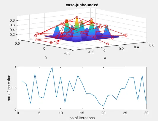
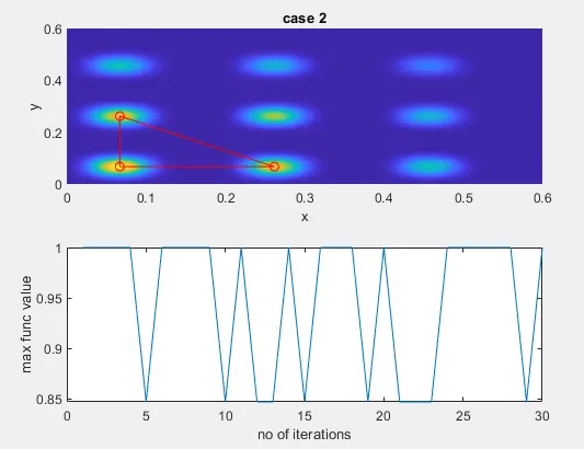
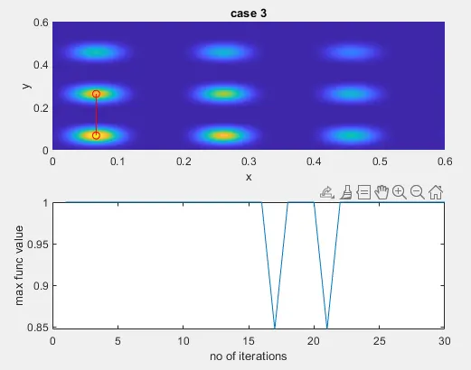
There are 3 cases that have been considered in this study-

1. Case 1- Unbounded (populationsize=50)

2. case 2-Bounded (Populationsize=50)

 

 

3. Case 3-Bounded (Populationsize=100)

 

 

4. Case 4-Bounded (Populationsize=300)

 

 

References :-  

1. https://en.wikipedia.org/wiki/Genetic_algorithm
2. https://in.mathworks.com/discovery/genetic-algorithm.html