Week 1- Mixing Tee
Aim:
- To set up steady-state simulations to compare the mixing effectiveness when hot inlet temperature is 360C & the Cold inlet is at 190C.
- Use of k-epsilon and k-omega SST model for the first case to analyze which is more suitable model for further cases.
- To try different cases for the given velocity and momentum ratio.
- To compare the values from the 2 cases such as cell count, Average outlet temperature, Number of iterations for convergence.
- To generate Velocity and temperature contour and line plots on the cut planes along and across the pipe.
- To Perform Mesh independent study for any one case.
- To Discuss the effect of length and momentum ratio on results.
Introduction:
Computational fluid dynamics (CFD) is a science that, with the help of digital computers, produces quantitative predictions of fluid-flow phenomena based on the conservation laws (conservation of mass, momentum, and energy) governing fluid motion. CFD has increased in importance and in accuracy; however, its predictions are never completely exact. Because many potential sources of error may be involved, one has to be very careful when interpreting the results produced by CFD techniques.The key to various numerical methods is to convert the partial different equations that govern a physical phenomenon into a system of algebraic equations.CFD is merely a tool for analyzing fluid-flow problems. If it is used correctly, it can provide useful information cheaply and quickly.finite-difference and finite-element methods and their applications are some methods used in CFD. There are other kinds of numerical methods also, for example, the spectral method and the spectral element method, which are often used in CFD. They share the common approach that discretizes the Navier-Stokes equations into a system of algebraic equations.
- Mixing tee: Mixing tee is a device which uses specifically engineered internal geometry to mix two fluid streams into one steam, efficiently.
- importance of using mixing tee:Turbulent mixing of fluid of different temperature in T-junction geometries became of significant importance in the field of nuclear reactor safety, since it can lead to highly transient temperature fluctuations at the adjacent pipe walls, cyclic thermal stresses in the pipe walls and consequently to thermal fatigue and failure of the pipeline. Thermal striping and mixing, in general, is however challenging to predict by using common CFD simulation and turbulence modeling approaches.
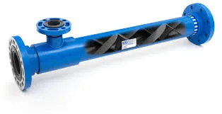
Static mixing tee
we are provided with two cases where we need to perform CFD analysis on both of them, they are:
- Case 1
- Short mixing tee with a hot inlet velocity of 3m/s.
- Momentum ratio of 2, 4.
- Case 2
- Long mixing tee with a hot inlet velocity of 3m/s.
- Momentum ratio of 2, 4.
Case-1_Short mixing tee
| hot Inlet velocity(m/s) | Momentum ratio | |
| analysis-1 | 3 | 2 |
| analysis-2 | 3 | 4 |
Case-2_long mixing tee
| hot Inlet velocity(m/s) | Momentum ratio | |
| analysis-1 | 3 | 2 |
| analysis-2 | 3 | 4 |
Formula:
Momentum ratio = velocity at cold inlet / velocity at hot inlet
1. 2= x/3;x=6m/s(velocity at cold inlet)
2. 4=x/3;x=12m/s(velocity at cold inlet)
Procedure:
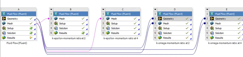
following below steps are for case 1, where one for k-epsilon and another for k-omega SST. Here, we are going to use the same geometry and mesh for both cases of analysis.
step 1: open Ansys workbench and click and drag fluent(fluid flow) to the workspace and double click on the geometry to open space claim and import short mixing tee model.
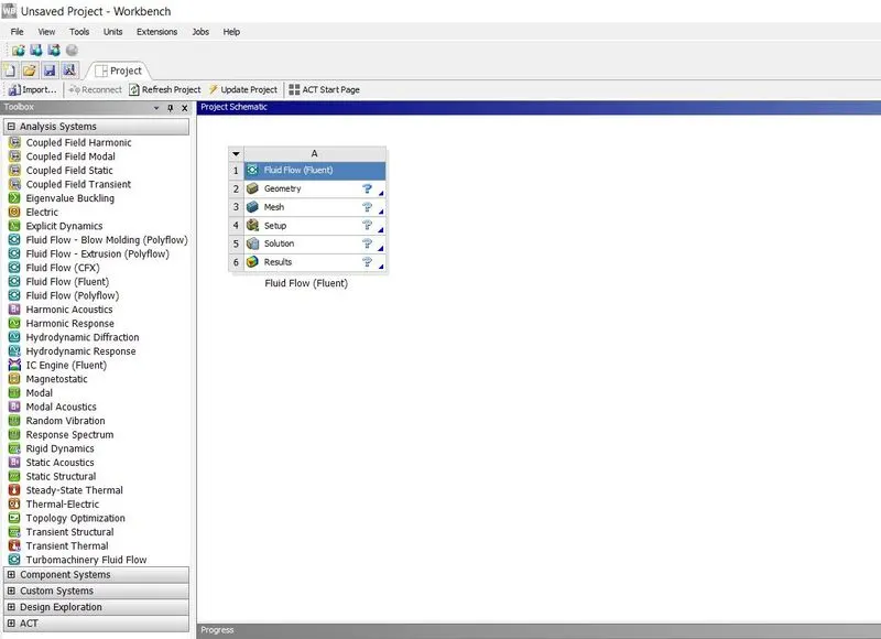
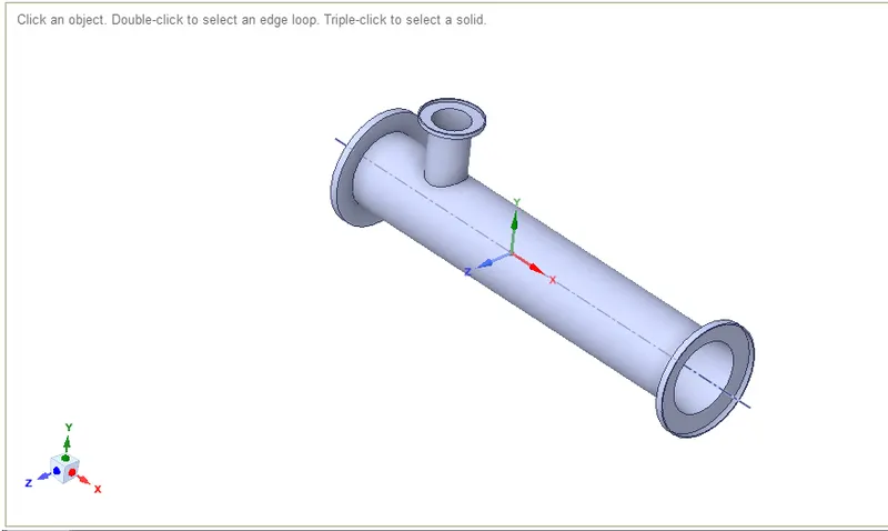
step 2: identify the surfaces where the fluid will interact and flow and create a volume and suppress the rest of the body.
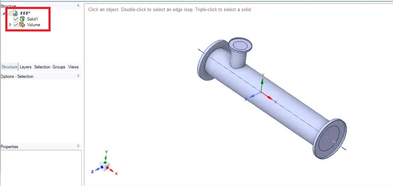
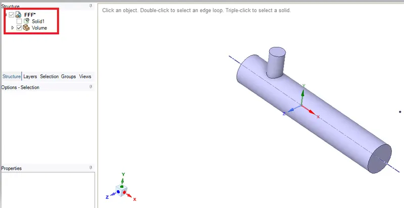
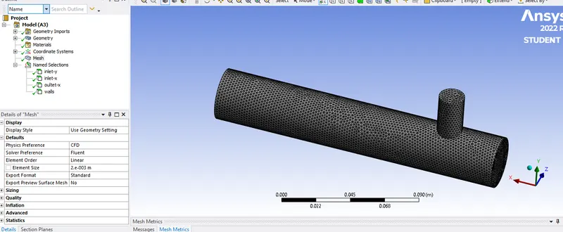
step 3: After creating a volume close the spaceclaim and go to workbench and double click on mesh, which will start Ansys meshing, where we can generate the mesh and assign names for inlet and oultet surfaces using name selection by selecting the face and pressing 'N' to assign the name for all the surface of the geometry.
here mesh element size= 0.002m and names as shown in below snap.
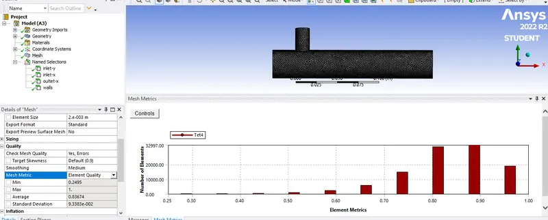
we can check our meshing by taking a cross section view And we can check the quality of mesh by clicking element quality as shown below to observe mesh flow.
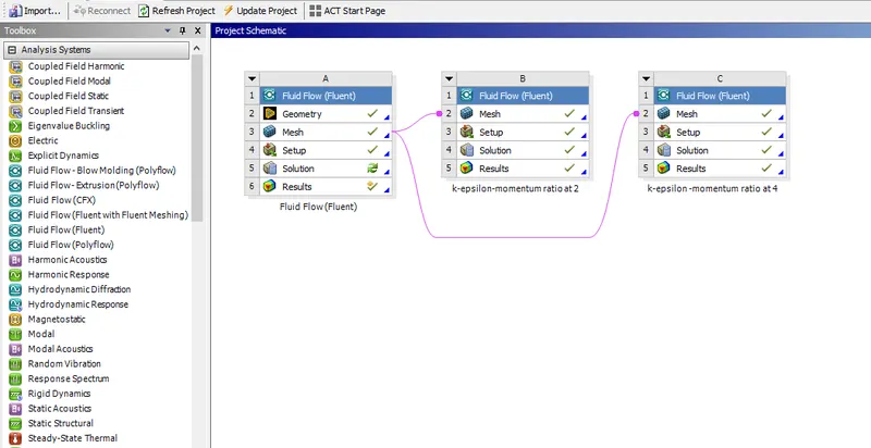
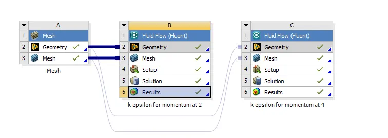
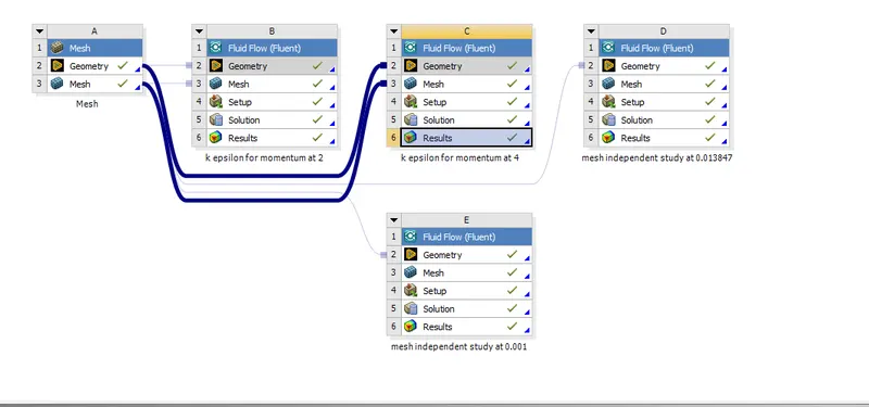
step 4: Here we use the geometry and mesh created.we can Drag the exiting mesh into the Fluent analysis Setup cell, one for k-epsilon-momentum ratio at 2 and other for k-epsilon -momentum ratio at 4. Then update the mesh (Right-click on mesh and use the update button) to convert and write the mesh for the FLUENT analysis.
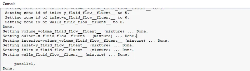
step 5: for k-epsilon-momentum ratio at 2, click on setup, there in the Fluent window, we will first see the console window which displays text, here we can use this console as text user interface also where all operations carried out in front and backend of the software will be be visible
After the complete loading of domain geometry, it will represent it in a graphical user interface, where can see the fluid flow in the geometry.
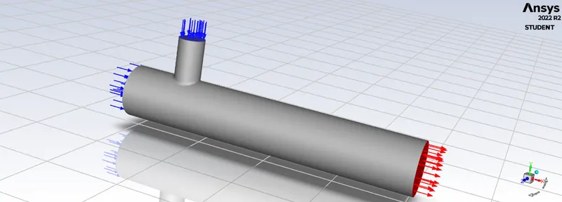
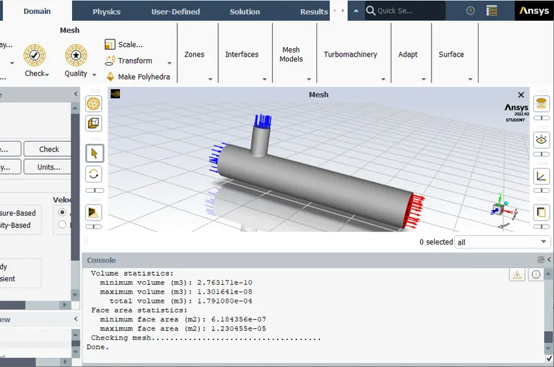
step 6: In the domain panel, we can check our mesh for fluent analysis and we can improve the quality using modify option.click on the check mesh quality button, it prints the analyzing in the console Window. The mesh check ensures that each cell is in a correct format and connected to other cells as expected. It is recommended to check every mesh immediately after reading it. Failure to check yields a badly formed or corrupted mesh that will need repairs prior to simulation.
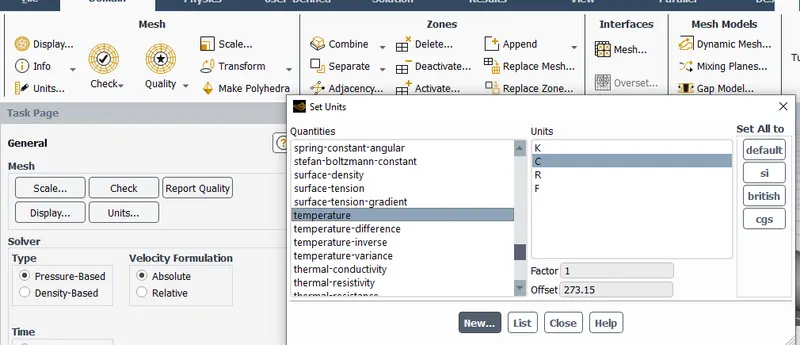
step 7:under domain, Click ‘units’ to change the unit of temperature.
step 8: click on physics.under general parameter setting we need to keep as it is. Solver type -> pressure-based; velocity formulation -> Absolute; solver time -> steady. 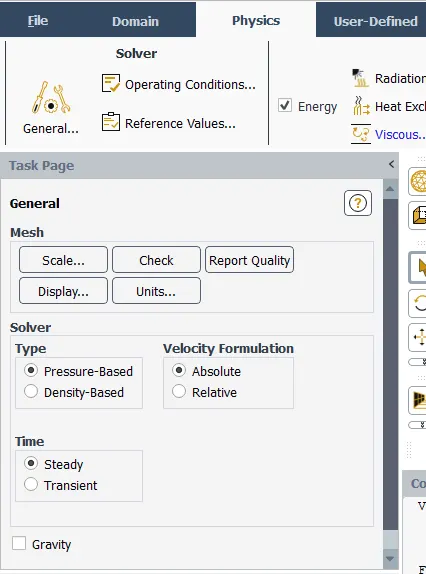
step 9:check-on energy Equation. since activating energy equation allows the temperature-dependent problem to be solved.

step 10: under viscous, select k-epsilon-Realizable’ for our first type of simulation.here we need to understand the meaning of k-epsilon and k-omega model, as said above we'll be comparing the both results of the turbulent models, since turbulence modeling is a complex area. The choice of model depends on the application.
The k-epsilon (k−ϵ) model for turbulence is the most common to simulate the mean flow characteristics for turbulent flow conditions. It belongs to the Reynolds-averaged Navier Stokes (RANS) family of turbulence models where all the effects of turbulence are modeled.k- epsilon model predicts well far from the boundaries (wall)
The K-omega model is one of the most commonly used turbulence models. It is a two equation model, that means, it includes two extra transport equations to represent the turbulent properties of the flow. This allows a two equation model to account for history effects like convection and diffusion of turbulent energy.K-omega model predicts well near the boundaries (wall).
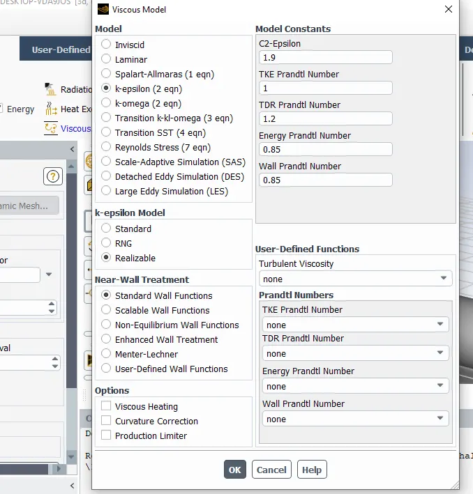
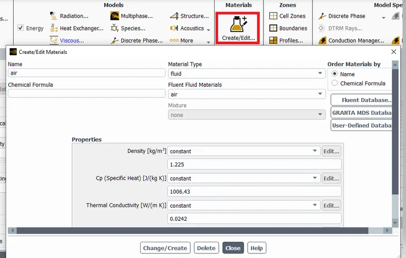
step 11: Now, select the materail which is required as fluid volume under materail option.our working fluid is air so we keep is as default material.
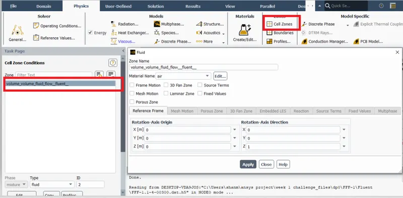
step 12: In the cell zone define the material, select the working fluid.
step 13:Now, we need to define the boundary conditions for each created name selection for inlet and oultet surfaces. following boundary conditions are inputted:
inlet-x- velocity=3m/s;temperature= 36 degree celsius.
inlet-y- velocity=6m/s;temperature= 19 degree celsius.(cold inlet velocity as per calculating momentum ratio as mentioned in above formula)
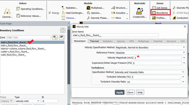
outlet-x will be considered as atmospheric pressure value which has zero gauge pressure and also there will be upstream influence in the turbulent model which will be bring back the turbulence in the flow, so in order to avoid we use honeycomb like structure.honeycombs are installed to straighten the flow against any
upstream influence.but in this model that is not the case so we can we can keep the backflow reference frame as absolute. 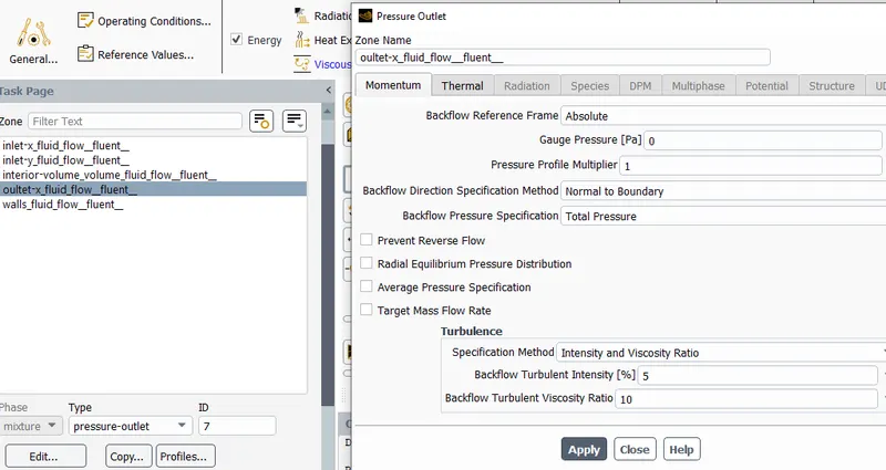
we need to repeat this step for different cold inlet velocity, they are as follows:
inlet-x- velocity=3m/s;temperature= 36 degree celsius.
inlet-y- velocity=12m/s;temperature= 19 degree celsius.(cold inlet velocity as per calculating momentum ratio as mentioned in above formula)
step 14: click on solution->definitions->new->area weight average and select the highlighted text as showm in below snapand press OK.
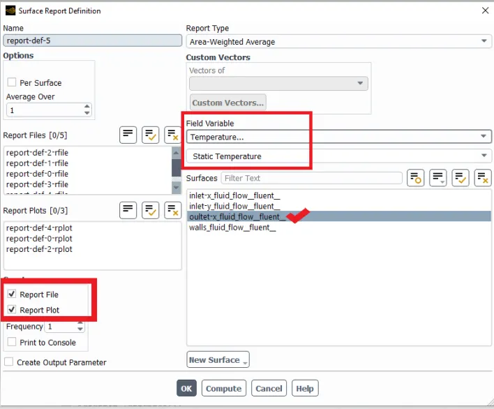
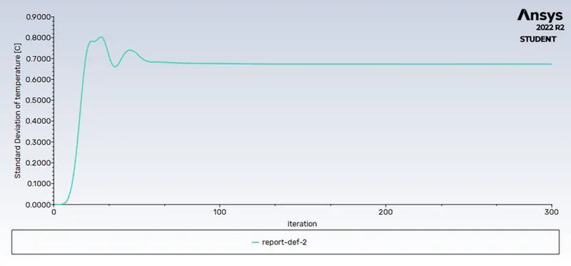
step 15: step 14 to be repeated for obtaining standard deviation which helps us to understand the effectiveness of mixing.
step 16: Now, Initialization is carried out to calculate approximate values of velocity, temperature and pressure.
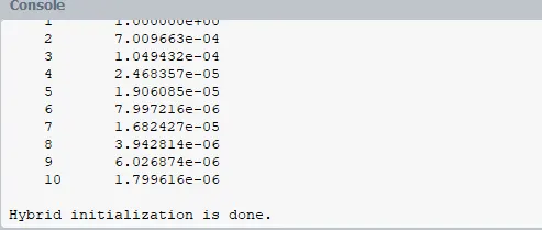
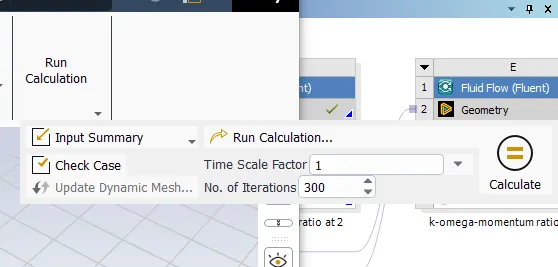
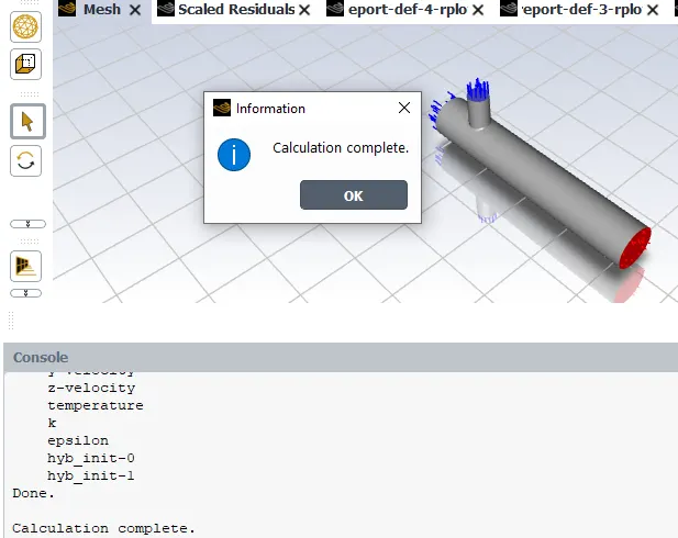
step 17:click on run calculator to input the no of iterations to 300 and click on calculate. If solution is not converged, then iterations can be increased.then we will a pop up saying calculation is complete.
step 18:close solution and go to workbench and double click on result to open CFD post. Check-in all the boxes to see walls and other parts and increase the transperency of the wall.
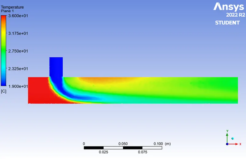
step 19: create a xy-plane at the wall in order view the temperature variation across the model and right click to edit and change it to by variable and to temperature.
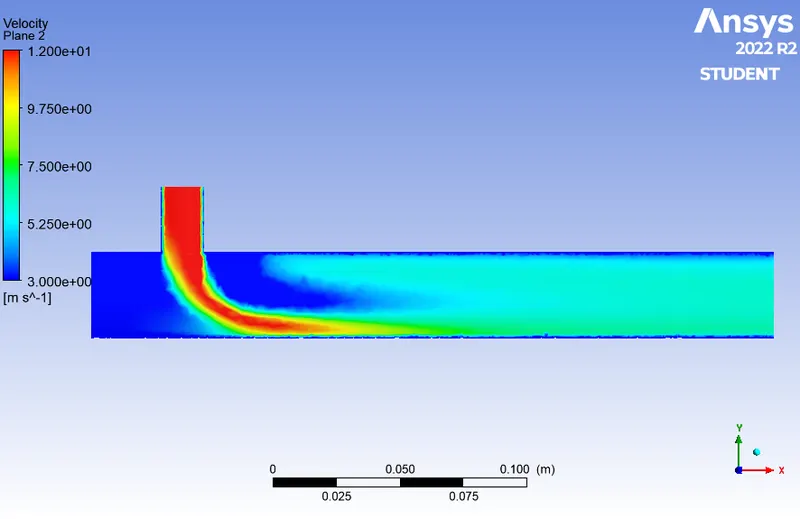
step 20: create another plane to view velocity variation across the model.
Note: This above procedure for simulation is followed for k-epsilon model, same procedure to be followed for k-omega SST model in case -1 and based on the assessment of the report on case-1, we can decide the use of the more suitable model for further cases.
Results:
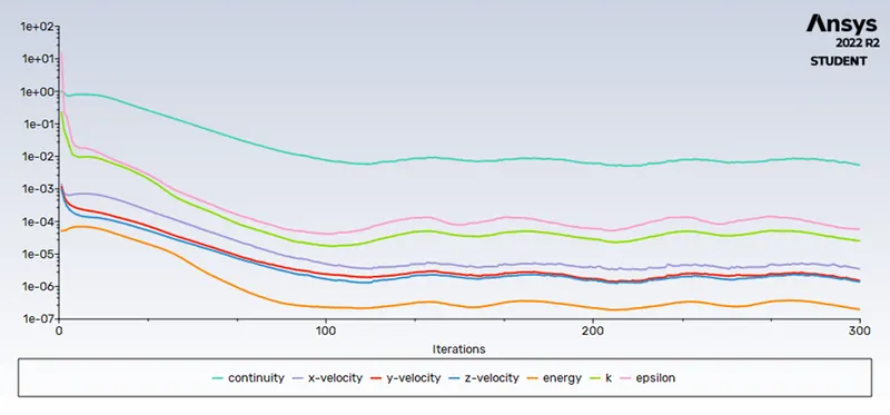
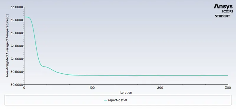
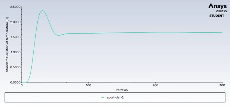
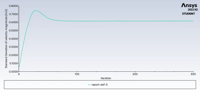
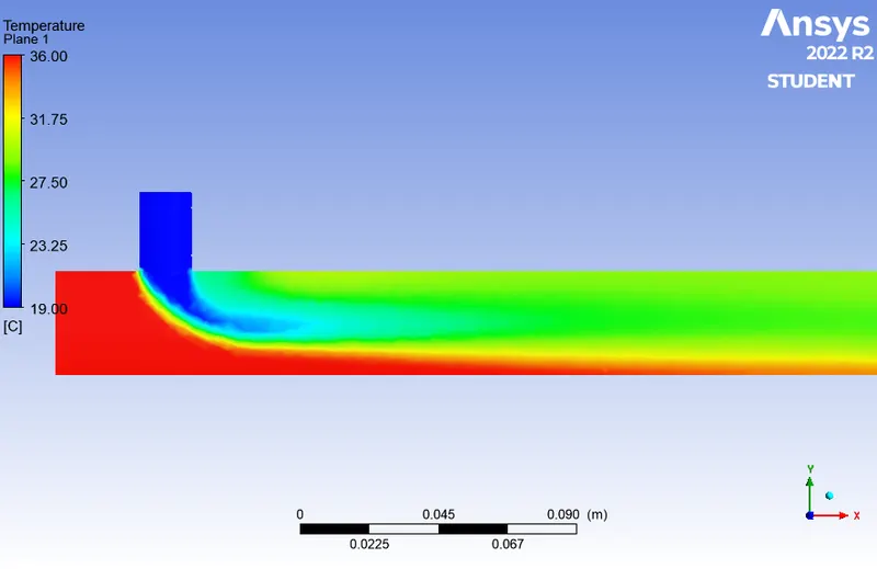
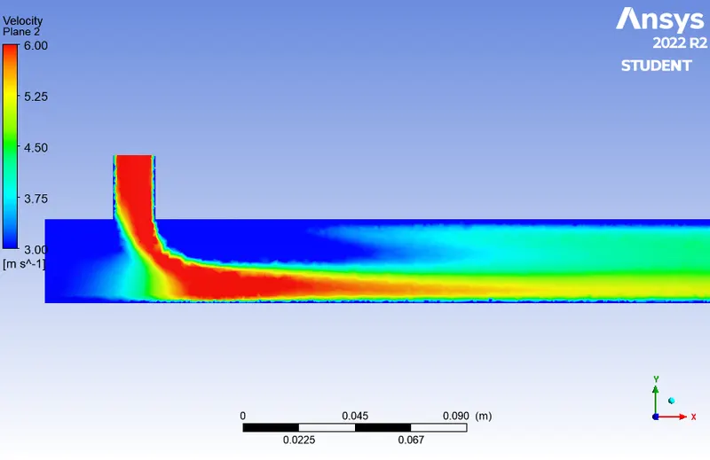
case 1: In this short mixing tee we considered hot inlet velocity inlet-x=3m/s at temperature=36 degree celsius; cold inlet velocity inlet-x=6m/s at temperature=19 for momentum ratio=2 and hot inlet velocity inlet-x=3m/s at temperature=36 degree celsius; cold inlet velocity inlet-x=12m/s at temperature=19 degree celsius for momentum ratio=4 degree celsius we used two different turbulent solvers such as k-epsilon, k-omega SST.
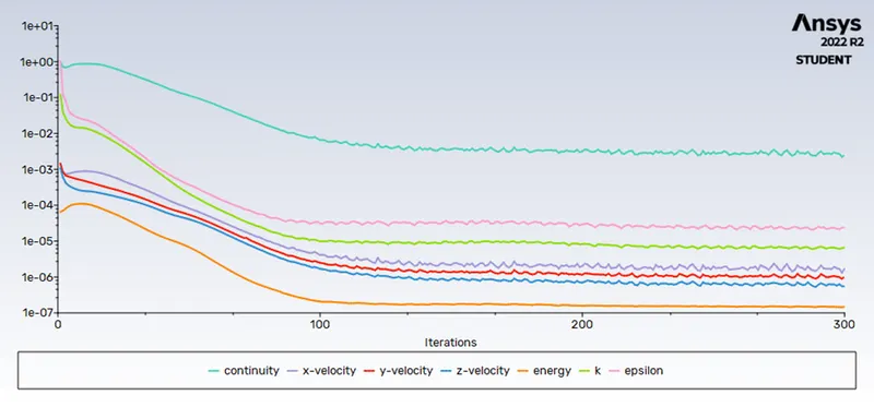
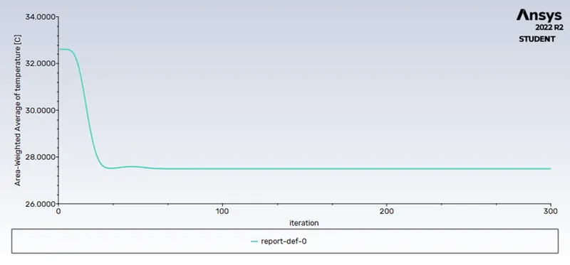
Plot and contours from k-epsilon model at velocity=3m/s;momentum ratio=2
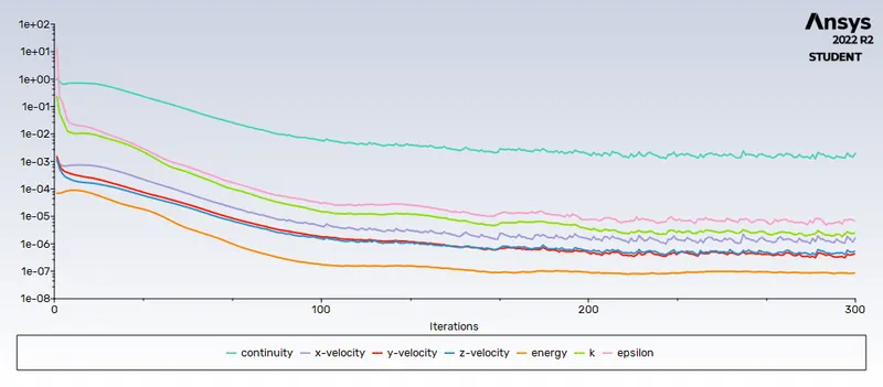
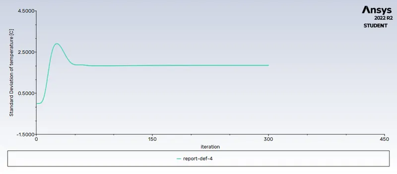
Residuals Standard Deviation of Temperature vs Iteration
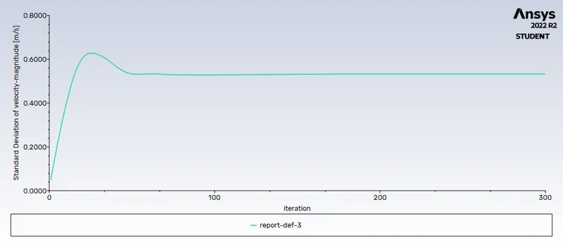
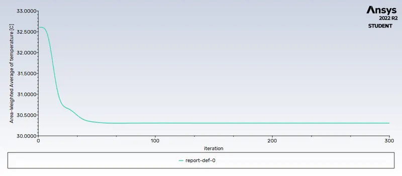
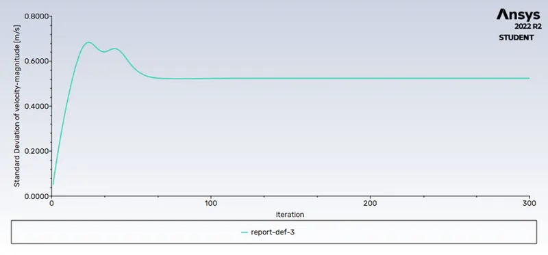
Standard Deviation of velocity vs Iteration Area-weighted Average Temperature vs Iterations
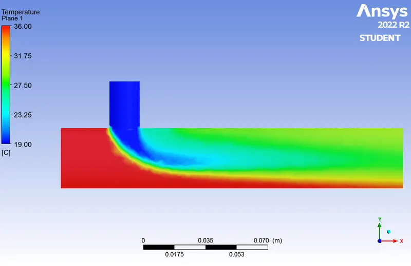
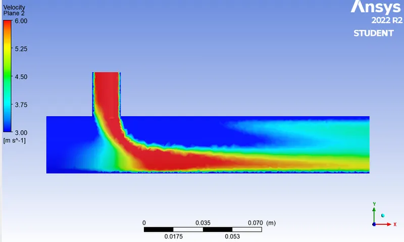
Temeprature Contour Velocity Contour
Plot and contours from k-epsilon model at velocity=3m/s;momentum ratio=4
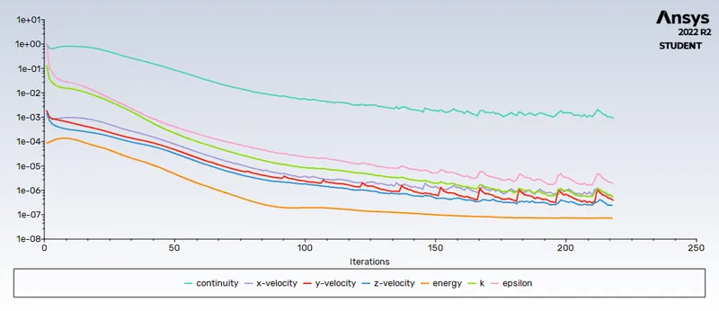
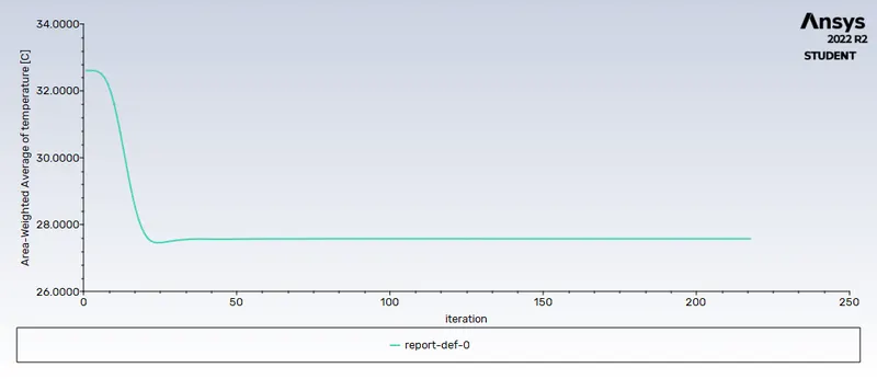
Residuals Area-weighted Average Temperature vs Iterations 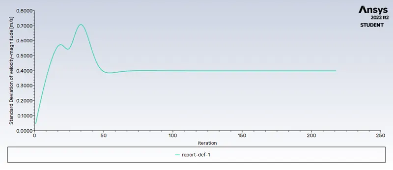
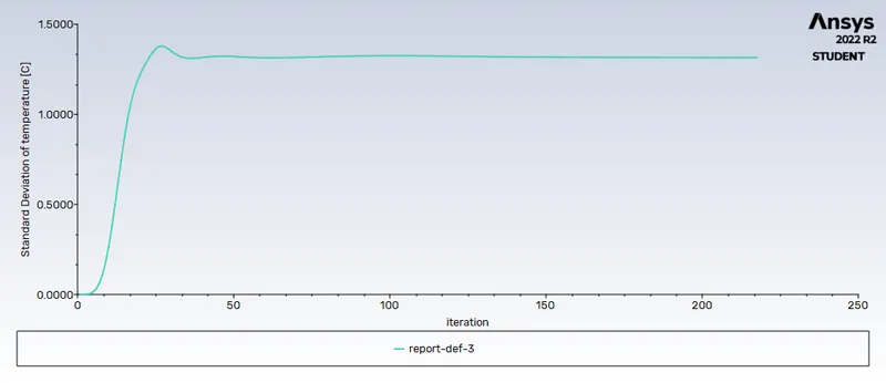
Standard Deviation of velocity vs Iteration Standard Deviation of Temperature vs Iteration
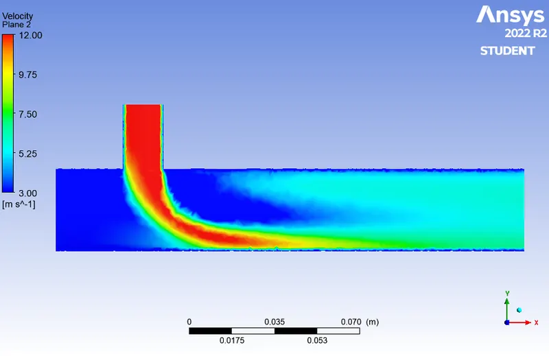
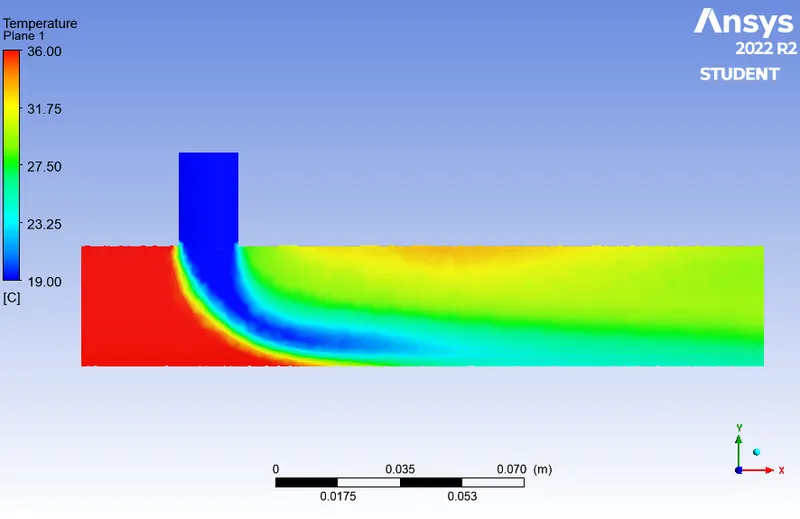
Velocity Contour Temeprature Contour
Plot and contours from k-omega model at velocity=3m/s;momentum ratio=2
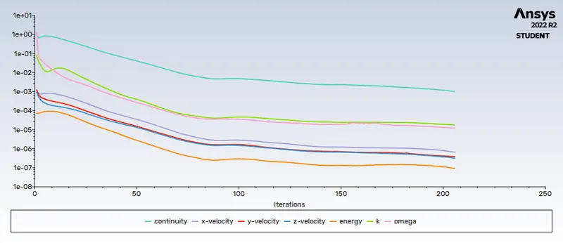
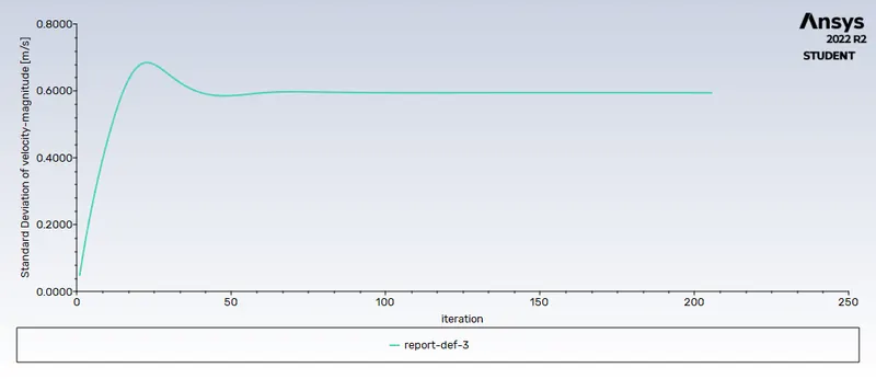
Residuals Standard Deviation of velocity vs Iteration
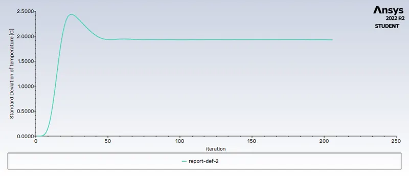
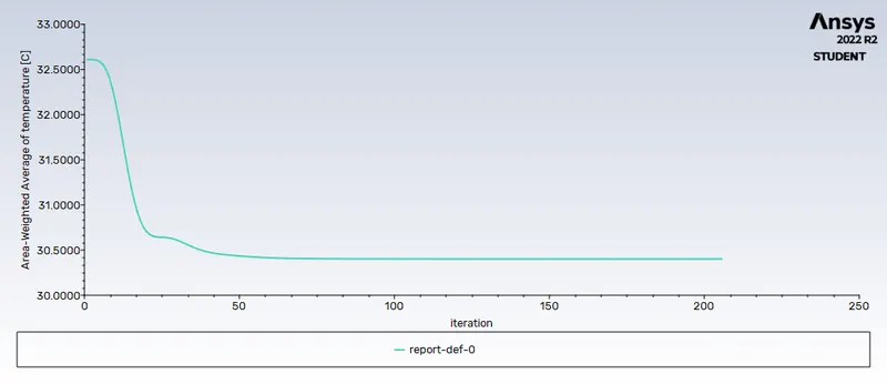
Standard Deviation of Temperature vs Iteration Area-weighted Average Temperature vs Iterations
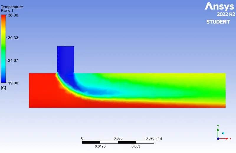
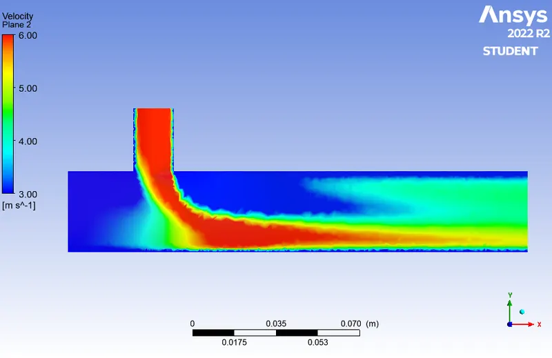
Temeprature Contour Velocity Contour
Plot and contours from k-omega model at velocity=3m/s;momentum ratio=4
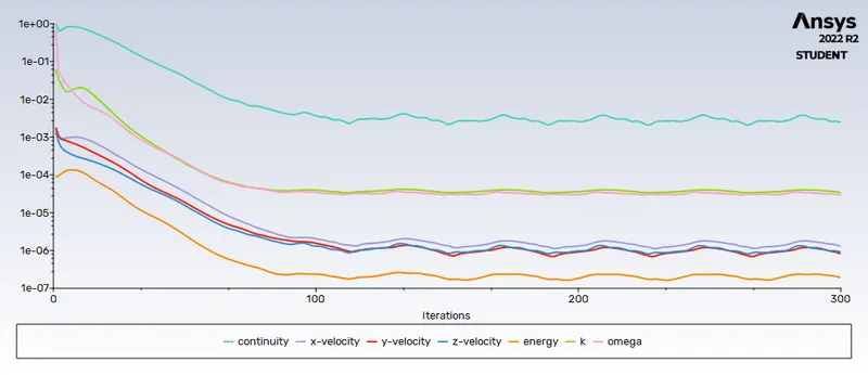
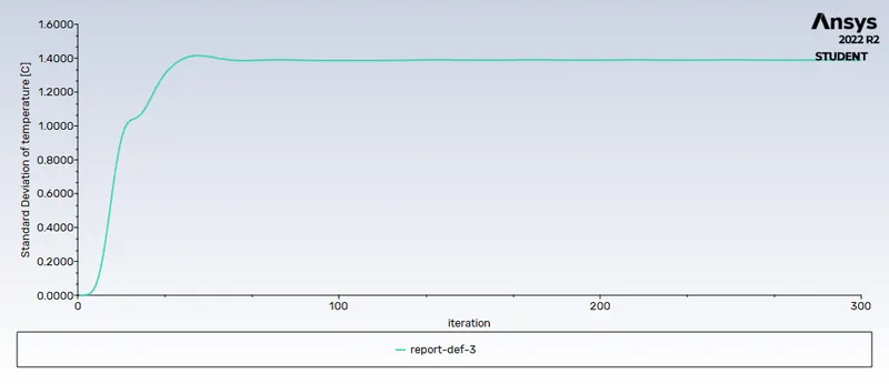
Residuals Standard Deviation of Temperature vs Iteration
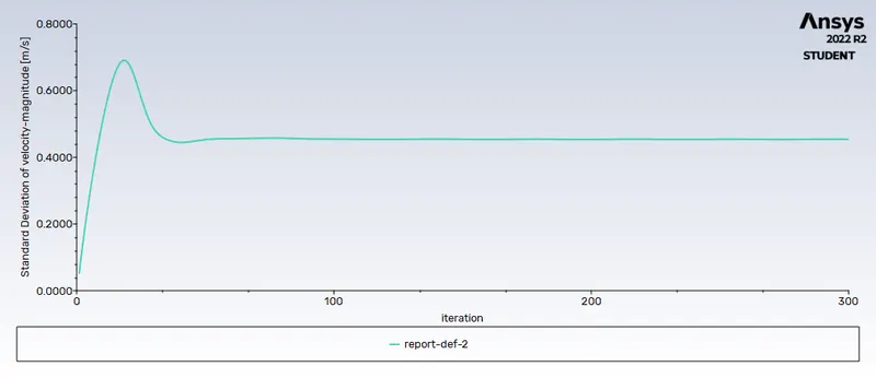
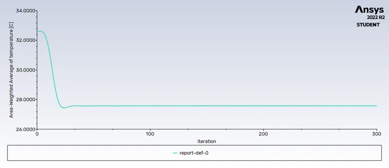
Standard Deviation of velocity vs Iteration Area-weighted Average Temperature vs Iterations
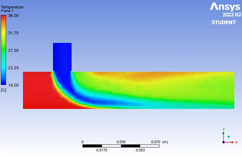
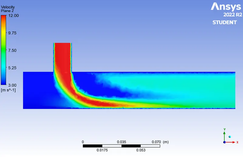
Temeprature Contour Velocity Contour
| Momentum Ratio=2 |
Cell count |
Average outlet temperature(degree celsius) |
No of iterations for convergence |
| CASE-1 |
106702 |
30.2968 | 298.025 |
| CASE-2 | 142758 | 30.3431 | 299.341 |
| Momentum Ratio=4 | Cell count | Average outlet temperature(degree celsius) | No of iterations for convergence |
| CASE-1 |
106702 |
27.5580 | 207.360 |
| CASE-2 | 142758 | 27.4838 | 300 |
After putting all the results in a single table we can compare our results where we can see the length of the mixing tee does not affect the results at the output that much if we ignore the diffusion criteria.
MESH INDEPENDENCE STUDY
The approach outlined above results in a single solution for the given mesh that we have used. Although we are happy that this has "converged" based on RMS Error values, we need to make sure that the solution is also independent of the mesh resolution. Not checking this is a common cause of erroneous results in CFD, and this process should at least be carried out once for each type of problem that we deal with so that the next time a similar problem arises, we can also apply the same mesh sizing.
The best way to check for a mesh independent solution is to plot a graph of the resultant residual value vs the number of iteration in your simulation. Here we will consider conducting mesh independent study for long mixing tee where three smiluations and analyzed whether the model is independent of mesh resolution as the mesh element size is refined.
By increasing the mesh size further we can see that the more number of cell simulation results in a value that is within my acceptable range. This indicates that we have reached a solution value that is independent of the mesh resolution,
Conclusion:
- steady-state simulations was setup to compare the mixing effectiveness when hot inlet temperature is 360C & the Cold inlet is at 190C.
- k-epsilon and k-omega SST model were used for the first case to analyze which is more suitable model for further cases decided that k-epsilon model for case-2.
- different cases were tried for the given velocity and momentum ratio.
- comparison between the values from the 2 cases such as cell count, Average outlet temperature, Number of iterations for convergence were carried out.
- Velocity and temperature contour and line plots were generated and analyzed on the cut planes along and across the pipe.
- Mesh independent study for were carried out for long mixing tee.
- the effect of length and momentum ratio on results were checked and analyzed.