Week 1- Mixing Tee
1. Aim:
The aim of the challenge is to created two versions of the mixing tee, One of them is longer than the other and perform pre-processing, solving and post processing to compare the velocity and temperature contour plots, mesh independent study and effect of length and momentum ratio on results.
2. Objective:
The main objective is to created two versions of the mixing tee. One of them is longer than the other and set up steady-state simulations to compare the mixing effectiveness when hot inlet temperature is 360C & the Cold inlet is at 190C. Using the k-epsilon and k-omega SST model for the first case and based on your judgment use the more suitable model for further cases and providing the reason for choosing a suitable model is mandatory. Comparing the cell count, average outlet temperature and number of iterations for convergence in a table.
- Case 1
- Short mixing tee with a hot inlet velocity of 3m/s.
- Momentum ratio of 2, 4.
- Case 2
- Long mixing tee with a hot inlet velocity of 3m/s.
- Momentum ratio of 2, 4.
Momentum ratio = velocity at cold inlet / velocity at hot inlet.
3. Introduction:
Mixing Tee CFD simulation
A branch of fluid mechanics called computational fluid dynamics employs math, physics, and computer software to simulate how fluids move through their medium and interact with their surroundings. Using governing equations such as the Navier-Stokes equation for momentum conservation, Consevation of mass and energy, computers are primarily used in CFD to predict fluid flow phenomena. The software Ansys Fluent will be used to simulate the influence of fluid in this investigation. In the field of CAE, Ansys Fluent is a crucial tool that enables you to carry out the three main processes of every simulation: pre-processing, solution, and post-processing. Ansys Fluent makes modelling flow, turbulence, heat transport, and chemical processes easier.
Mixing Tee is a T-joint because it splits the flow and angle between them is 90 degree. In mixing tee outside air comes through one side and chilled air comes inside the other inlet. Now by adjusting the flow rate of the chilled air we can get desired temperature at the outlet of the mixing tee which would be connected at the air conditioned system. This work flow of the mixing tee is simulated through the ANSYS workbench. There are set of process to find the reults. Spaceclaim to design the geometry, Mesh, Setup fluent and Setup CFD post processing.

4. Solving & Modelling approach:
Any type of simulation may be carried out in three main processes, which are as follows:
- Pre-processor, which comprises geometry cleanup and mesh generation of the highest quality.
- Boundary conditions, initialization, and convergence are all components of solving.
- The next phase is post processing, which includes creating plots, contours, and vectors to analyse the findings.
Case-1
Short mixing tee
a - Simple mesh
hot Inlet velocity - 3m/s
Momentum ratio - 2,4
Case-2
Long mixing tee
a - Fine mesh with element size of 0.001
hot Inlet velocity - 3m/s
Momentum ratio - 2,4
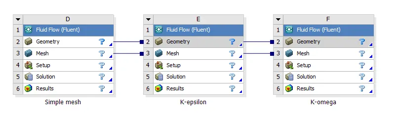
Drag and drop the ANSYS-Fluent in the ANSYS workbench.
Let us start with analyzing the best method to converge the solution for this particular case by studying two methods: k-epsilon and k-omega SST.
Now click on geometry to import mixing tee model. It will redirect to Spaceclaim, Ansys’s geometry model manipulator.
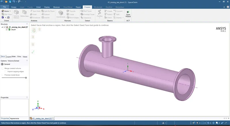
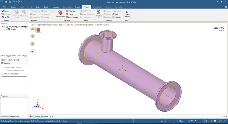
Spaceclaim plays a huge role in time consuming process of supressing the unwanted surfaces. To extract the fluid volume, go to prepare and select the volume extract to extract the fliud volume. By using select edge method to extract the fluid volume, select the edges to create a new volume for simulation.
Hiding the solid component to visualize the new volume and supress for the physics option.
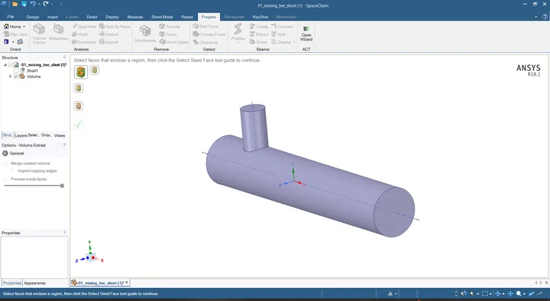
Close the spaceclaim and proceed to the meshing process.
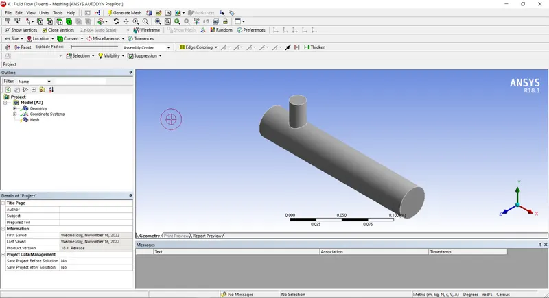
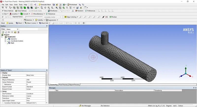
Initially generate the mesh and check the element quality.
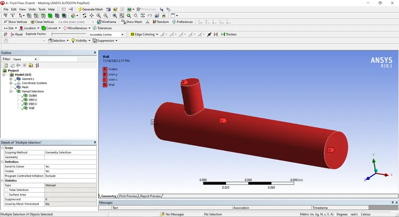
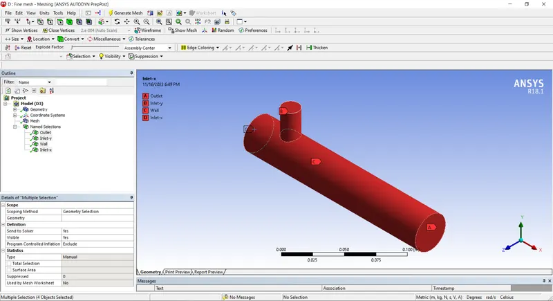
Select outer face and press right click of mouse, it will open a menu. Click on option create named selection and write suitable name for face.
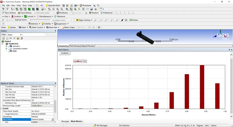
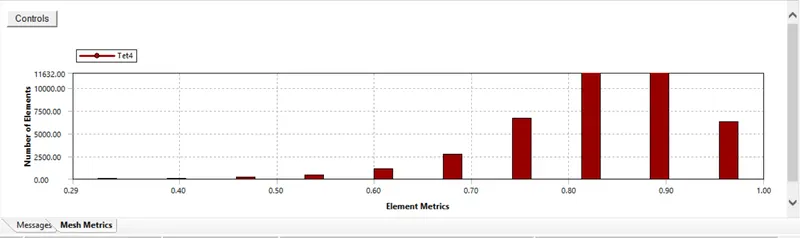
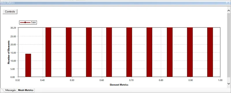
Select the option element quality to see, how many elements are defying quality. Quality is measured on the scale of 0 to 1. The number of element vs element metrices show the quality is near 1. So, it is considered as good quality.
Close the mesh interface and open the setup and solving the given criteria. Start solving the model first check the mesh.
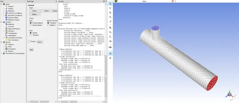
The below table represent the boundary condition given to check which model is suitable for analysis. First K-epsilon is used for the analsyis.
| Model | K-epsilon |
| Mesh type | Simple |
| Mixing tee | Short |
| Hot inlet velocity | 3m/s |
| Hot inlet temperature | 360C |
| Cold inlet temperature | 190C |
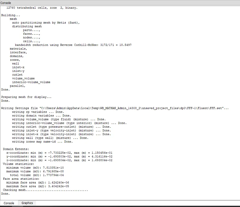
After opening the setup, first step is to check the mesh.
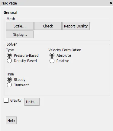
We are going to do pressure based steady state simulation, so choose these options on task page.
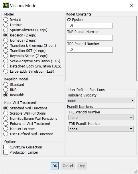
Go to physics menu and select viscous model. It will open a menu, choose realizable k-epsilon model and close it.
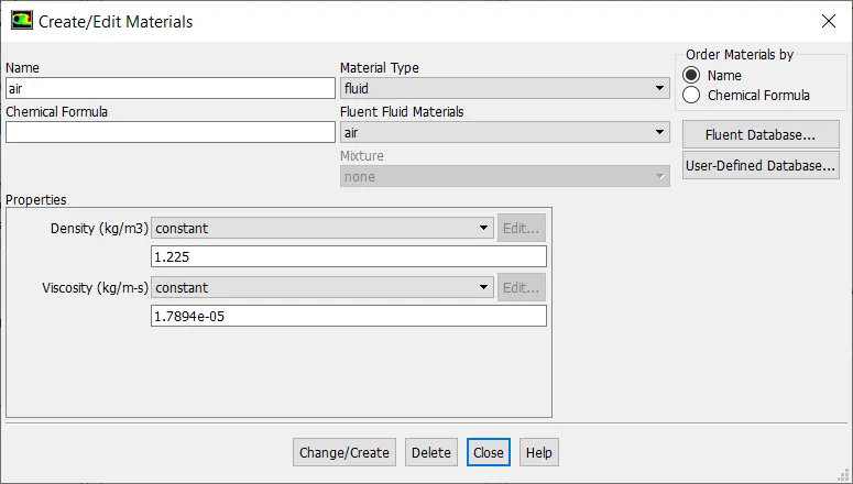
Click on materail and choose air as working fluid. Check working fluid by clicking on cell zone conditions option, if it is air then proceed.
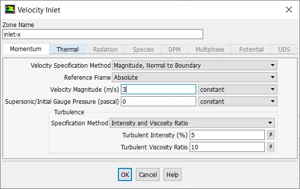
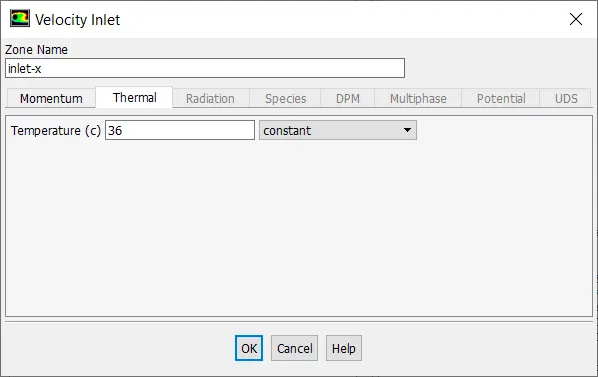
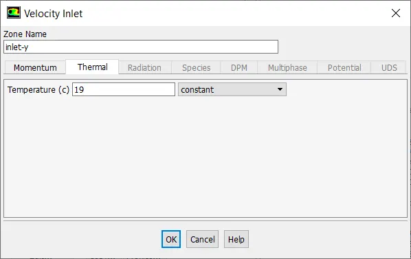
Now providing the hot inlet velocity 3m/s because its momentum ratio is 2 and hot inlet temperature is 36 degree celcius.
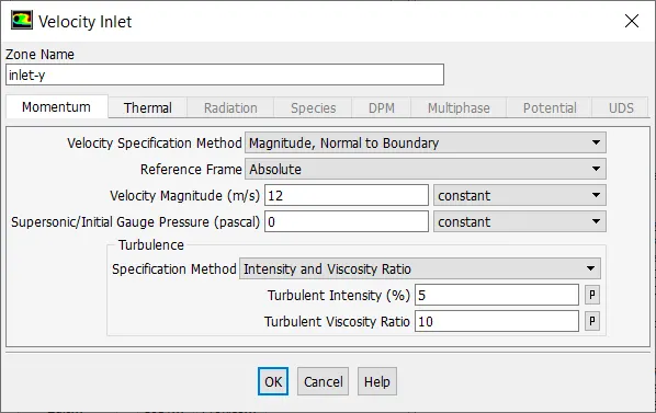
Now providing the hot inlet velocity 12m/s because the momentum ratio is 4 and cold inlet temperature is 19 degree celcius.
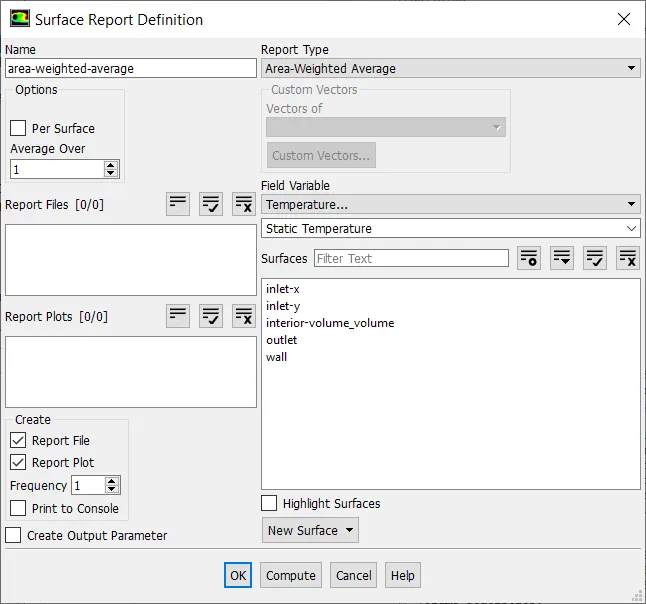
Defining the area-weighted average to the model.
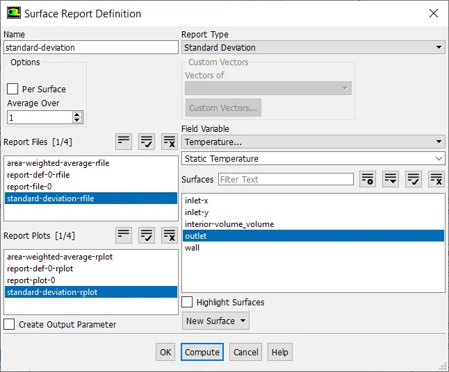
Defining the standard deviation to the outlet.
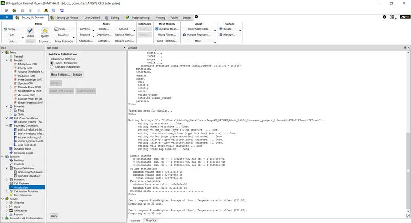
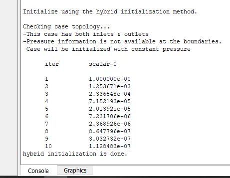
Then initialize the solution.
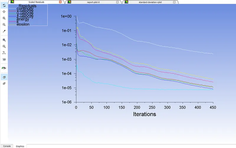
The below are the residulas, area-weighted average of temperature and standard deviation of temperature. The number of iteration is 150.
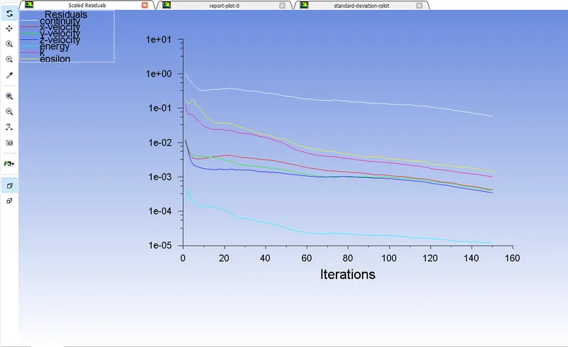
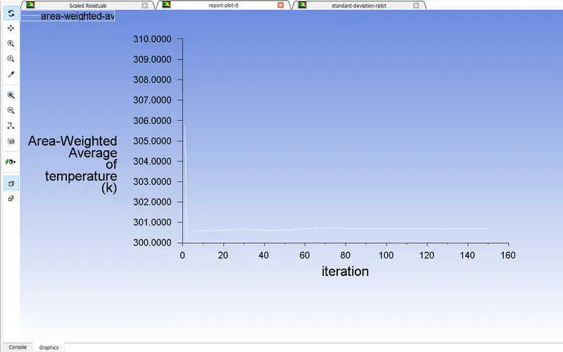
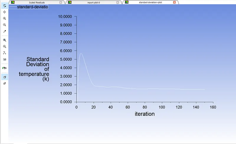
The below are the residulas, area-weighted average of temperature and standard deviation of temperature. The number of iteration is 300.
After this, we can close the fluent and post-process the results. Click on the results in the workbench and it will open CFD-Post.
CFD-Post initially displays the outline (wireframe) of the model which can be turned on by checking the surface shown in the Outline panel in the fluid section.
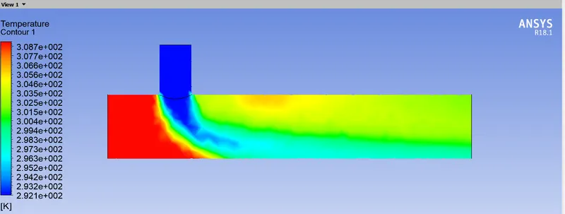
Temperture Contour:
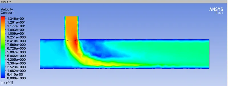
Velocity contour:
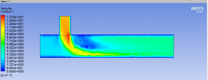
Similarly the solving process is done for the k-omega model and comparing the results.
| Model | K-omega |
| Mesh type | Simple |
| Mixing tee | Short |
| Hot inlet velocity | 3m/s |
| Hot inlet temperature | 360C |
| Cold inlet temperature | 190C |
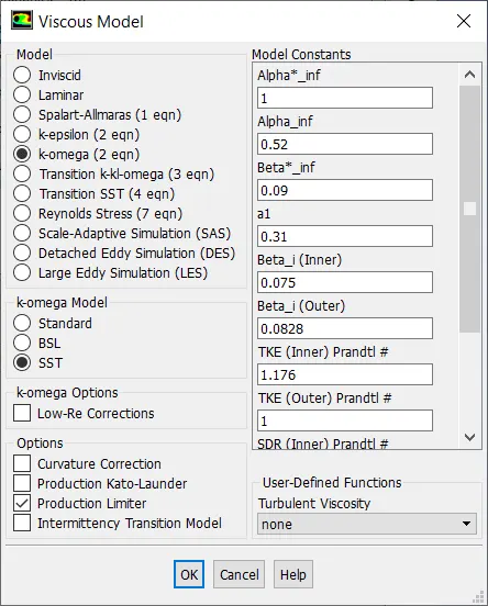
Go to physics menu and select viscous model. It will open a menu, choose K-omega SST model and close it.
Now providing the hot inlet velocity 3m/s because its momentum ratio is 2 and hot inlet temperature is 36 degree celcius.
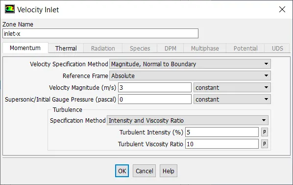
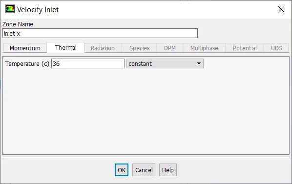
Now providing the hot inlet velocity 12m/s because the momentum ratio is 4 and cold inlet temperature is 19 degree celcius.
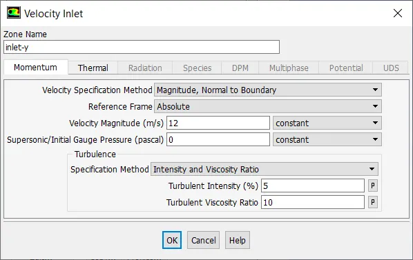
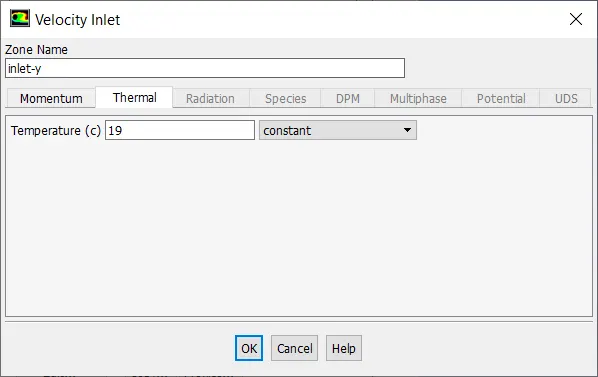
Defining the area-weighted average to the model and standard deviation of the model.
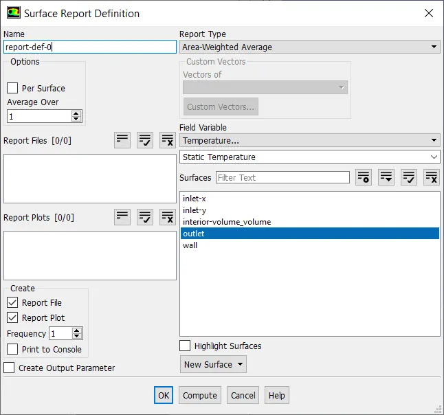
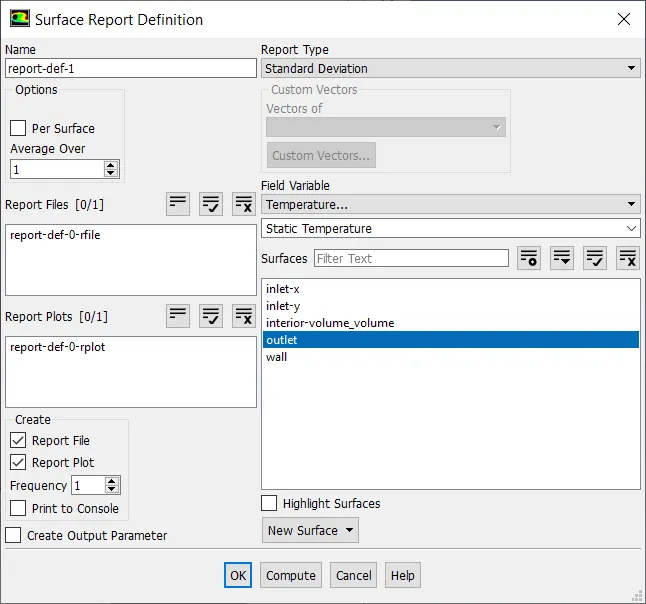
Initializing the calculation.
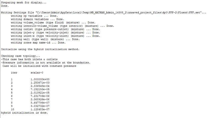
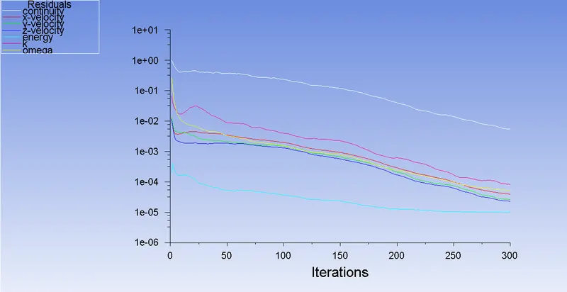
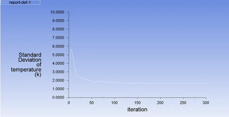
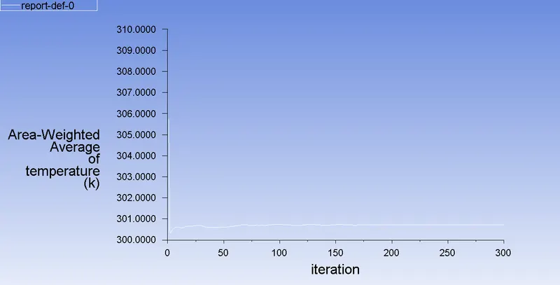
The below are the residulas, area-weighted average of temperature and standard deviation of temperature. The number of iteration is 150.
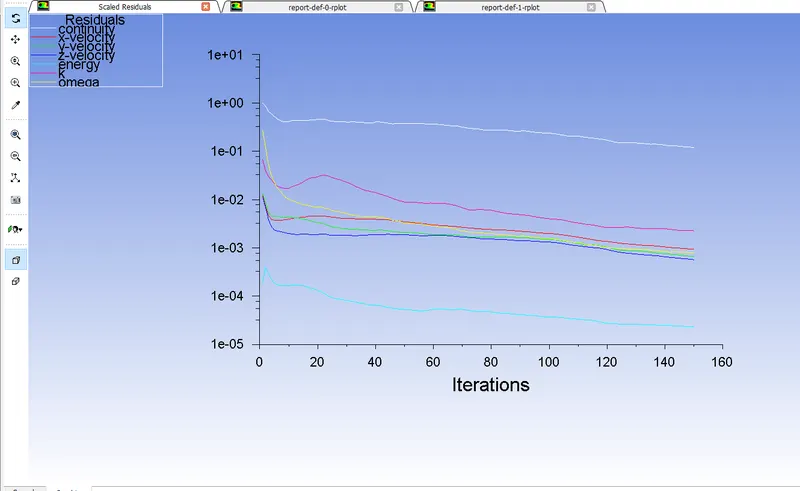
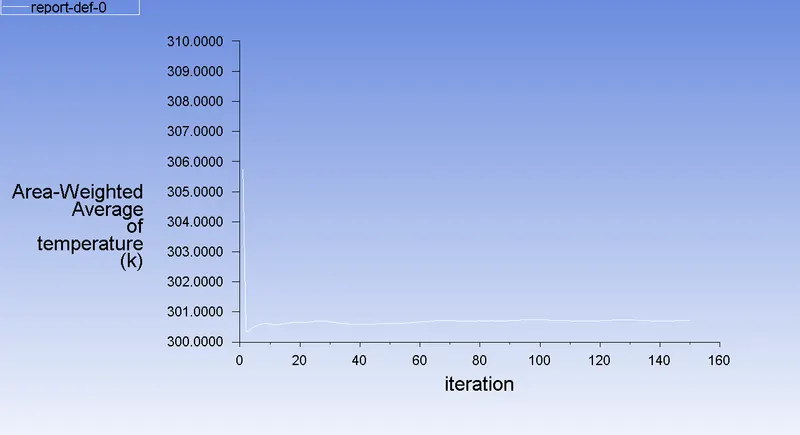
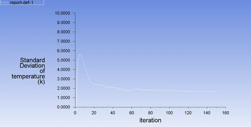
The below are the residulas, area-weighted average of temperature and standard deviation of temperature. The number of iteration is 300.
After this, we can close the fluent and post-process the results. Click on the results in the workbench and it will open CFD-Post.
CFD-Post initially displays the outline (wireframe) of the model which can be turned on by checking the surface shown in the Outline panel in the fluid section.
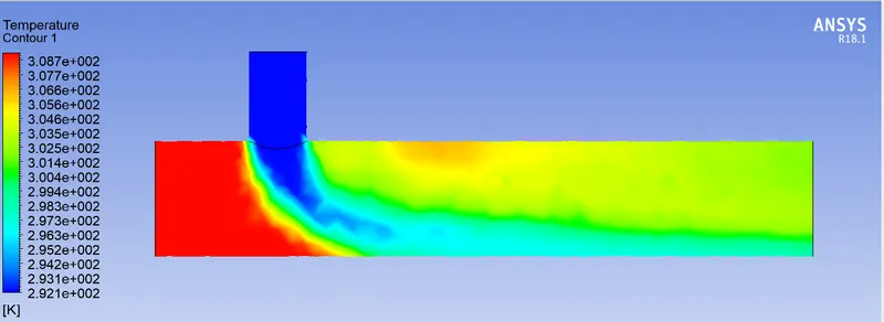
Temperture Contour:
Velocity contour:
The reason for choosing a suitable model:
K-epsilon model:
The most popular model used in CFD to simulate mean flow properties under turbulent flow conditions is the K-epsilon turbulence model. It is a two-equation model that uses two transport equations to describe turbulence (PDEs). The rate of dissipation of turbulent kinetic energy (k) is the second transferred variable after turbulent kinetic energy (k), which are the first two carried variables.
K-omega model:
Many aerodynamic applications utilize the SST k-omega turbulence model, which is a two-equation eddy-viscosity model. The k- omega model is well suited for simulating flow in the viscous sub-layer.
Difference between two models:
K-epsilon model - temperature contour K-omega model - temperature contour
The viscous sub-layer flow may be accurately simulated using the k- omega model. The k-epsilon model, however, excels in predicting flow in areas far from the wall. Compared to many other turbulence models, the SST model is less sensitive to free stream conditions (Flow outside the boundary layer). The k-omega model is assisted by the shear stress limiter in preventing an accumulation of excessive turbulent kinetic energy close to stagnation spots. If we check at our simulation figure, we can see that the k-omega model's flow is more laminar and does not provide suitable turbulent outcomes, whereas the k-epsilon model's simulation produces proper mixing of the two air streams.
Reason for selelcting k-epsilon model:
K-epsilon is producing superior results since the solution converged after only a few iterations, but the solution was not converged when using the K-omega model. In investigating fluid behaviour near to walls, K-omega is preferable, however this is not the case here. Therefore, in future cases, the k-epsilon model is recommended for the analysis of fluid in the flow region that is away from the wall.
Finally, the model is decided for the next long mixing tee model.
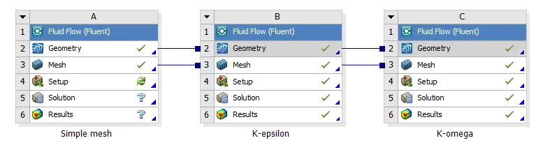
Then, analysing the mixing tee for below considerations.
| Model | K-epsilon |
| Mesh type | Fine mesh of element size of 0.001 |
| Mixing tee | Short |
| Hot inlet velocity | 3m/s |
| Hot inlet temperature | 360C |
| Cold inlet temperature | 190C |
1. Importing the extractcted the fluid volume to the geometry.
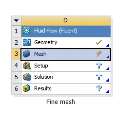
2. Open the mesh interface and give the element size as 0.001 and generate mesh.
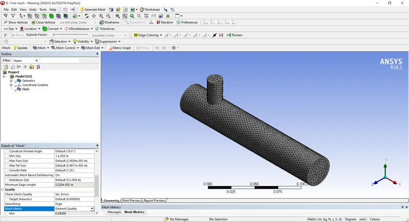
Element metrics vs number of elements is given below.
Naming the sections as inlet, outlet and wall.
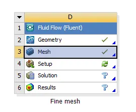
Fine mesh is done for the mixing tee model.
Open the setup and provide the necessary boundary conditions for the model.
Now providing the hot inlet velocity 3m/s because its momentum ratio is 2 and hot inlet temperature is 36 degree celcius.
Now providing the hot inlet velocity 12m/s because the momentum ratio is 4 and cold inlet temperature is 19 degree celcius.
Defining the area-weighted average to the model and standard deviation of the model.
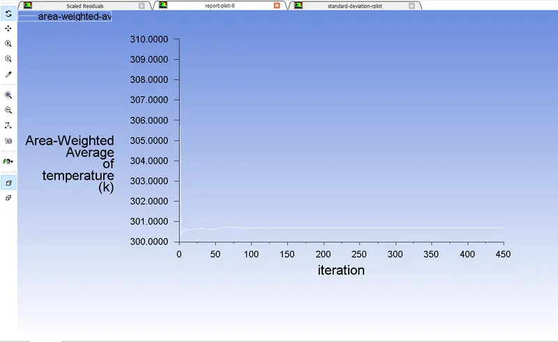
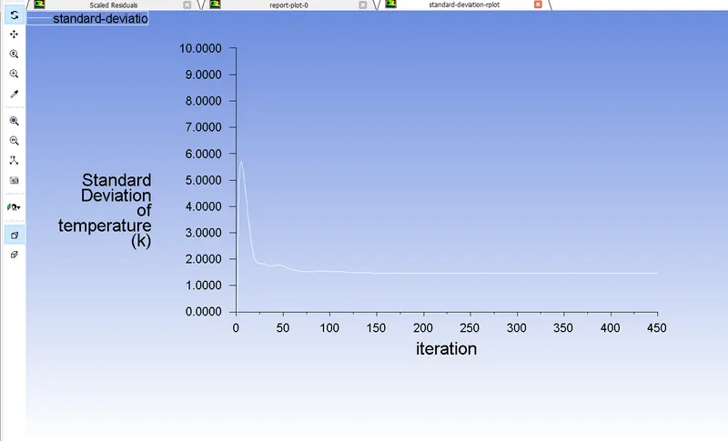
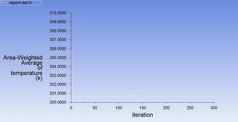
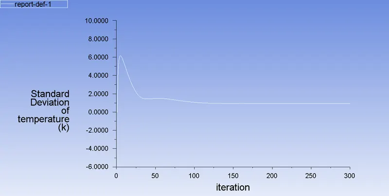
The below are the residulas, area-weighted average of temperature and standard deviation of temperature. The number of iteration is 300.
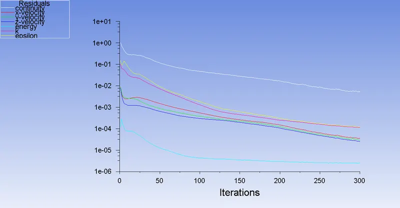
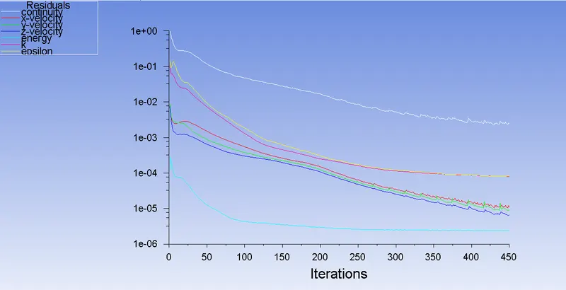
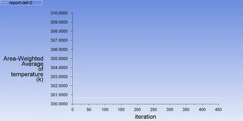
The below are the residulas, area-weighted average of temperature and standard deviation of temperature. The number of iteration is 450.
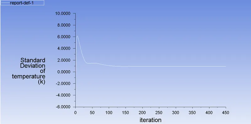
After this, we can close the fluent and post-process the results. Click on the results in the workbench and it will open CFD-Post.
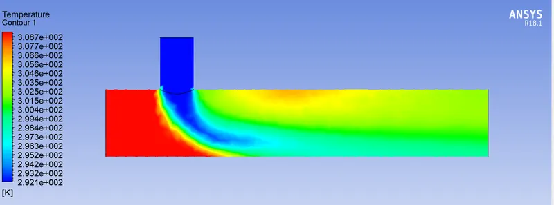
CFD-Post initially displays the outline (wireframe) of the model which can be turned on by checking the surface shown in the Outline panel in the fluid section.
Temperture Contour:
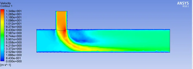
Velocity contour:
Finally, all the process is done for the short mixing tee.
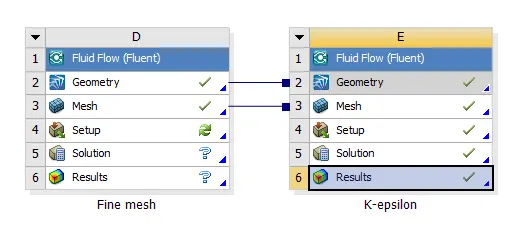
Then, analysing the mixing tee for below considerations.
| Model | K-epsilon |
| Mesh type | Fine mesh of element size of 0.001 |
| Mixing tee | Long |
| Hot inlet velocity | 3m/s |
| Hot inlet temperature | 360C |
| Cold inlet temperature | 190C |
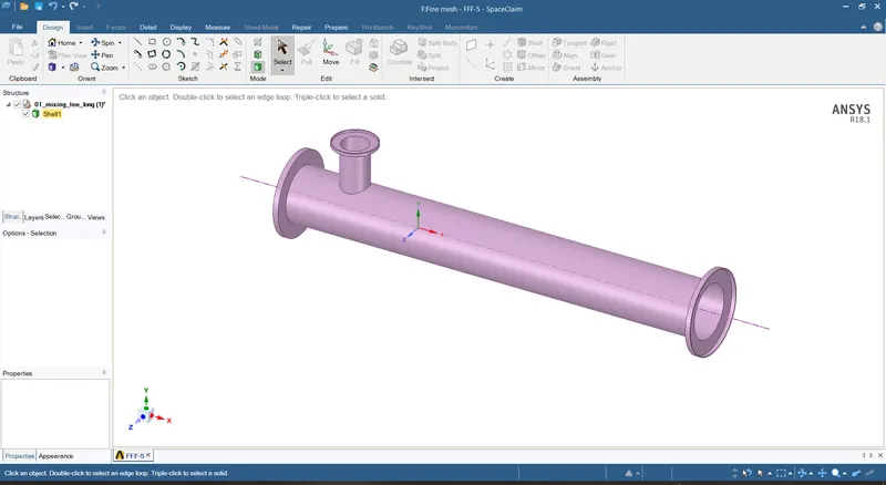
Importing the geometry and open in the spaceclaim and supress the unwanted surface.
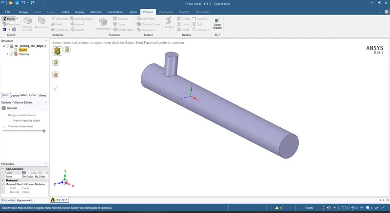
This is the extracted volume for the analysis.
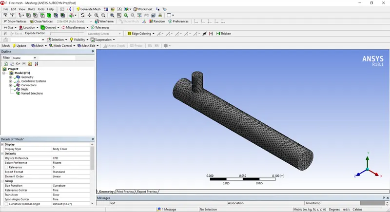
Open the mesh and provide the necessary fine mesh to the model.
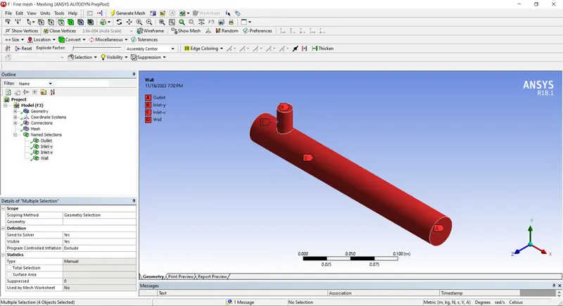
Naming the surface for the setup process.
Quality check for the meshing.
Open the setup and provide the necessary boundary conditions for the model.
Now providing the hot inlet velocity 3m/s because its momentum ratio is 2 and hot inlet temperature is 36 degree celcius.
Now providing the hot inlet velocity 12m/s because the momentum ratio is 4 and cold inlet temperature is 19 degree celcius.
Defining the area-weighted average to the model and standard deviation of the model.
The below are the residulas, area-weighted average of temperature and standard deviation of temperature. The number of iteration is 300.
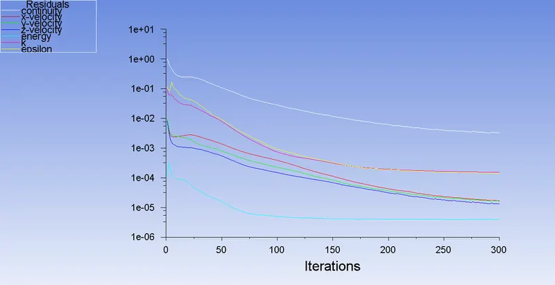
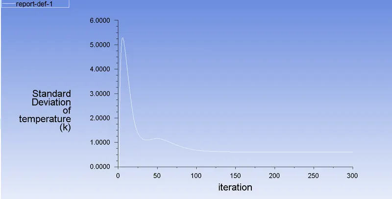
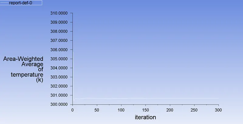
The below are the residulas, area-weighted average of temperature and standard deviation of temperature. The number of iteration is 450.
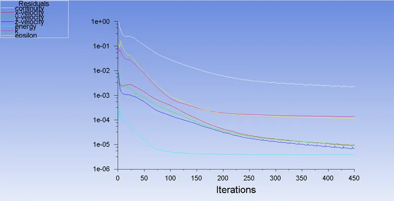
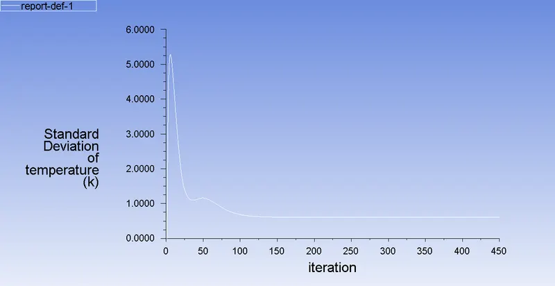
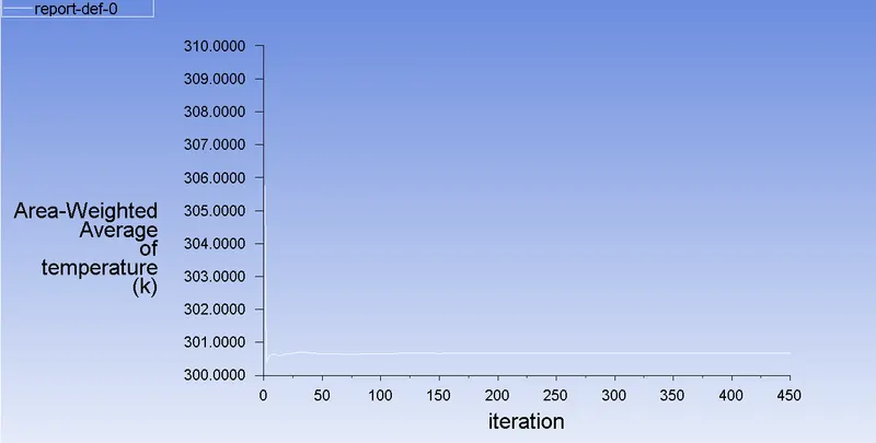
After this, we can close the fluent and post-process the results. Click on the results in the workbench and it will open CFD-Post.
CFD-Post initially displays the outline (wireframe) of the model which can be turned on by checking the surface shown in the Outline panel in the fluid section.
Temperture Contour:
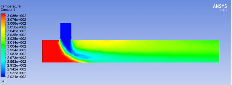
Velocity contour:
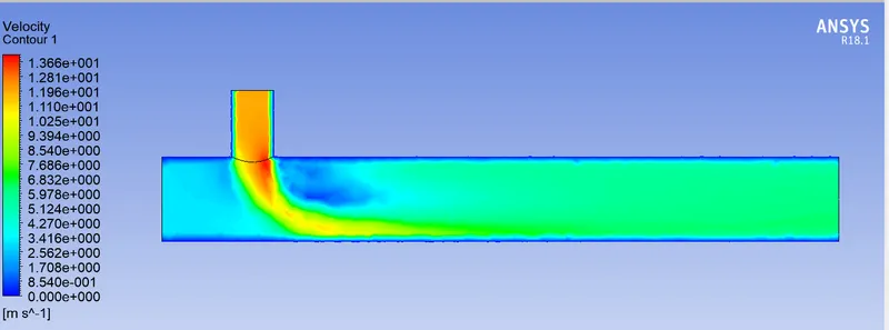
Results:
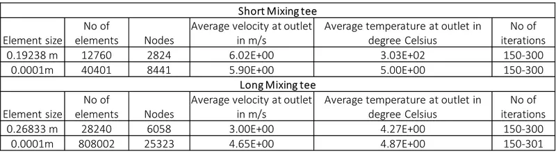
Conclusion:
High flow velocity can improve mixing at the outlet very effectively. As a result, a larger momentum ratio results in improved fluid stream mixing at the outflow.
Diffusion flow always results in somewhat better mixing of two fluids, hence the length of the mixing tee increases.
The k-omega model predicts flow close to the wall, whereas k-epsilon models suggest flow essentially far from the boundary (wall).
The k-epsilon method is used because in this situation we require a flow simulation turbulence model far from the wall.
Finally, in the above cases, it is essential to have the right a short mixing tee with a momentum ratio of 4, but one must also take into account the flow diffusion over the length of the mixing tee; in this instance, a long mixing tee with momentum will be a better choice.