Week 1- Mixing Tee
MIXING TEE (Theory & It's Application)
Fluids are transported through flow sections. Flow sections of circular cross sections are known as pipes. Most fluid especially liquids are transported in circular pipes. This is because, pipes with a circular cross section can withstand large pressure differences between the inside and outside without significant distortion.
A typical piping system involves pipes of different diameters connected to each other by various fittings (T-Junction, Y-Junction) or elbow to ensure continuous transport of the fluid. In tee-Joint Frictional losses could occur in pipe flow. Added to that with the difference in temperature of the fluid passing through the inlets (x and y axis) could create certain changes in the temperature of the flow when mixing happens.
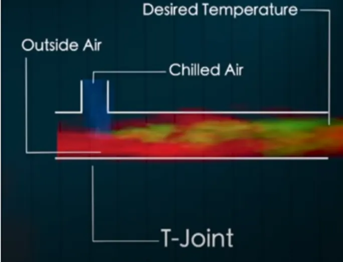
Mixing problems, such as the design and scale-up of a mixer and quantification of mixing, have been traditionally tackled by developing empirical design equations mainly due to the complexity of the fluid dynamics of mixing. Although this approach has proven to be satisfactory for many applications, it is rather limited because it neglects the complexity of flow in most mixing applications.
Applications where pipeline mixing with tees is used include low viscosity mixing such as wastewater treatment and blending of some oils (injection of additives) and petrochemical products. Other applications include blending of fuel gas, and mixing of feed streams for catalytic reactors. A tee is formed by two pipe sections joined at a right angle to each other. One stream passes straight through the tee while the other enters perpendicularly at one side.
Tee pipes are commonly used in piping systems and multi-channel network in various industries like electronic, petrochemical, nuclear plant etc, the mixing of hot fluid and cold fluid give rise to temperature fluctuation in the vicinity of mixing zone. The flow pattern of fluid gives necessary information such as area, where thermal zones are high. Using different momentum ratio, the efficiency of the model and its effectiveness is checked.
AIM:
To set up steady-state simulations to compare the mixing effectiveness when hot inlet fluid & the cold inlet fluid mix together using mixing tee.
GIVEN:
Hot inlet temperature = 360C
Cold inlet temperature = 190C
01_mixing_tee_short.SLDPRT
01_mixing_tee_long.SLDPRT
Hot Inlet Velocity = 3m/s
Momentum ratio 2
Momentum ratio 4
Momentum ratio = velocity at cold inlet / velocity at hot inlet
EXPECTED OUTCOMES:
Use the k-epsilon and k-omega SST model for the first case and based on your judgment use the more suitable model for further cases.
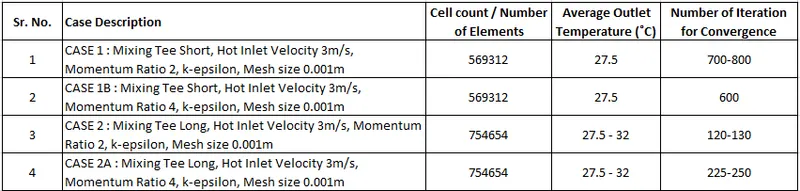
In a table, compare the following values from the 2 cases.
- Cell count
- Average outlet temperature
- Number of iterations for convergence
Velocity and temperature contour plots on the cut planes along and across the pipe.
Perform Mesh independent study for any one case.
Discuss the effect of length and momentum ratio on results.
OBJECTIVE:
- Understand and define the problem statement for each case.
- Open the Ansys workbench and set up a Fluid Flow (Fluent) simulation setup, and rename it accordingly.
- Under Fluid Flow (Fluent) setup, open space claims by clicking Geometry, and then load the given geometry. Extract the working fluid region from the loaded geometry to compute simulation in that particular region and then close the space claim.
- Next, under Mesh boundary names are assigned for each surface and generate mesh to the fluid flow volume. Close the mesh setup and update the mesh.
- Later, in the setup section, provide all the required parameters according to the simulation, such as simulation type, input velocity and temperature, materials (working fluid), and other user-defined parameters.
- In setup parameters, understand the concept of k-epsilon and k-omega SST and find out which is convenient for the current simulation.
- Afterward, simulate our problem setup for the number of iterations required to converge our results.
- Then, close and update the setup. Open the results section to see all the simulated results.
- Bring together the generated results from each case for their cell count, average outlet temperature, and the number of iterations for convergence.
- Display a contour plot on the cut plane to visualize velocity and temperature distribution along and across the mixing tee’s length.
- Validate the test by performing a mesh independence study on any one case.
- Study the effect of length and momentum ratio on the results of each case.
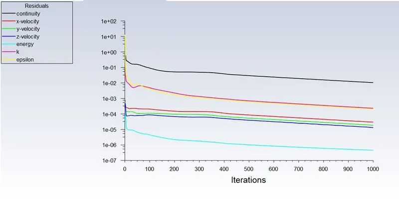
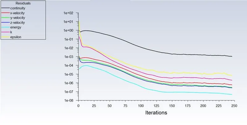
- Plot the convergence graph to verify that all the results are fully converged after running numerous iterations.
STEPS USED FOR SIMULATIONS
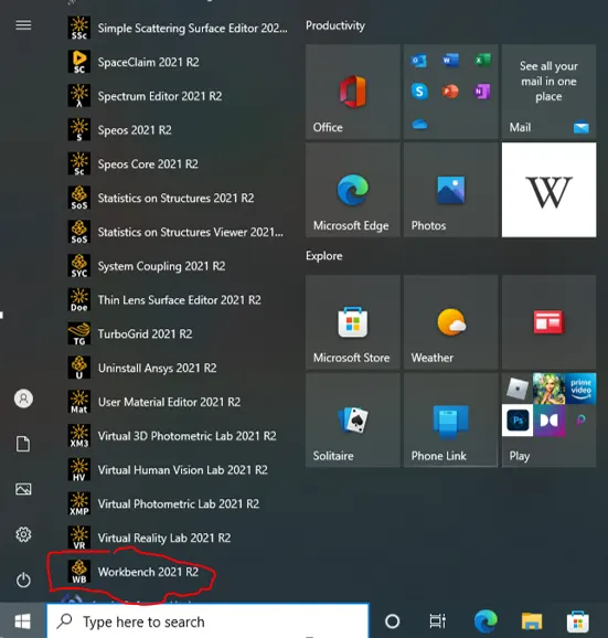
Click on red encircled "Workbench 2021 R2" as shown in the above image to start the simulation.
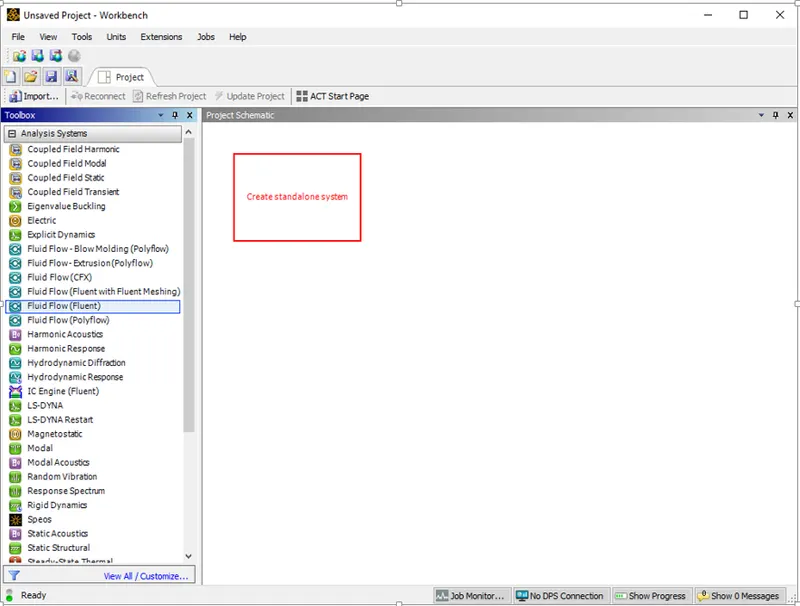
Click On Fluid Flow (Fluent) under Analysis Systems and drag it to create a standalone system.
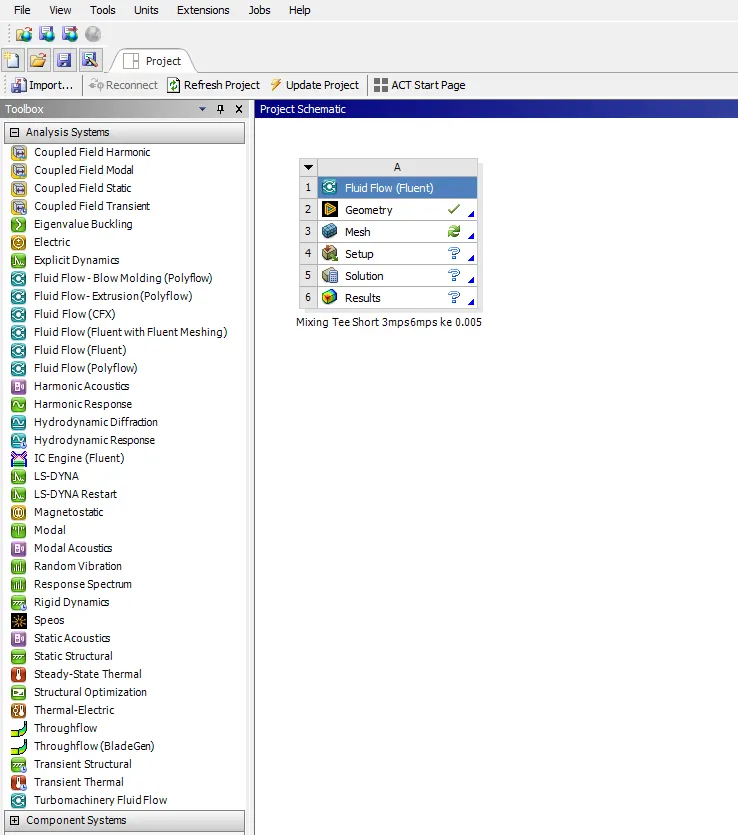
Rename the Project by using the left click and then click the Geometry.
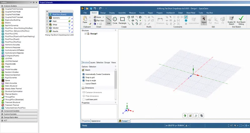
On clicking the geometry the space claim window opens as shown in the above image where we can create the geometry or load the existing geometry.
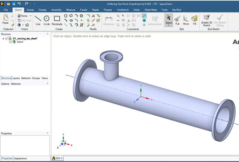
01_mixing_tee_short.SLDPRT is loaded in the space claim as shown in the above figure. In this geometry we are looking for the internal flow analysis as are simulating the mixing effectiveness of hot fluid and cold fluid.
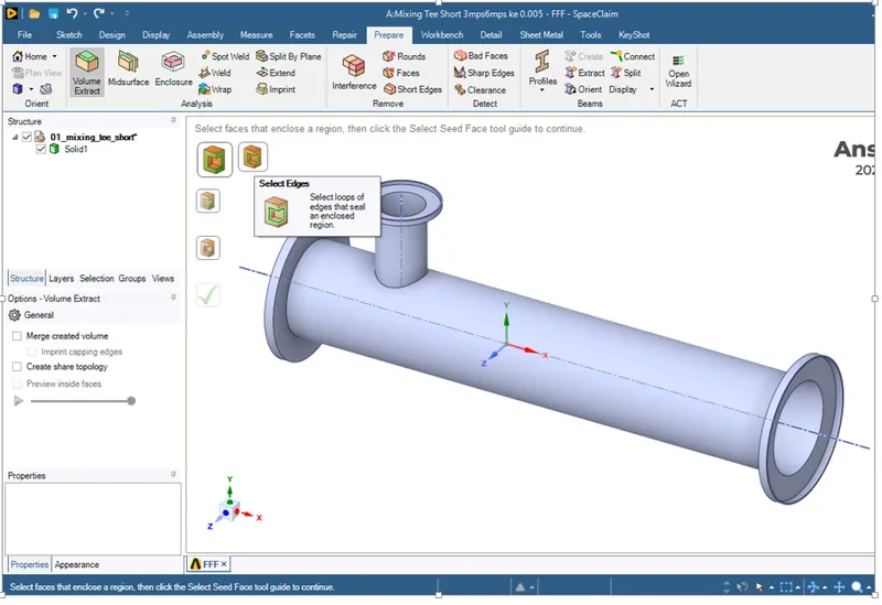
We need to extract the internal volume, we prepare the geometry for simlulations by extracting the internal volume. Internal vome is extracted using the select edges as shown in the above image.
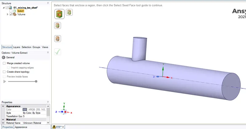
The internal volume is extracted as shown in the above image, the remaing part of the geometry is hidden by unclicking the tick on the part tree available at the left hand side. We also suppress the remaing part of the geometry for physics. Once this is done we close the geometry.
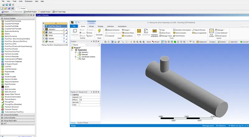
On clicking the Mesh the window opens where we can do the meshing.
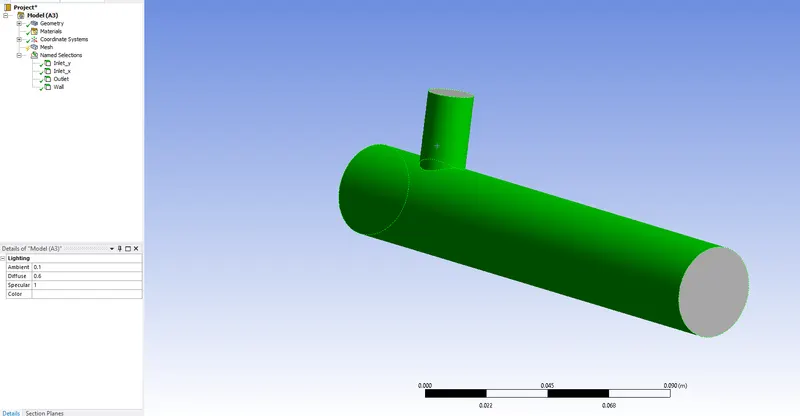
We give the names for the different entity where we can apply the boundary conditions. the options used is Named selection.
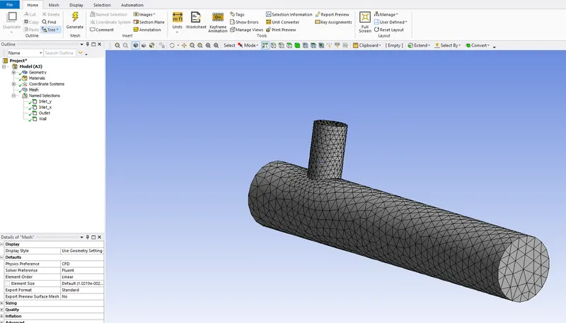
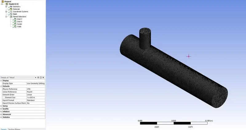
On clicking the generate, a mesh is created with default element size as shown in the above image.
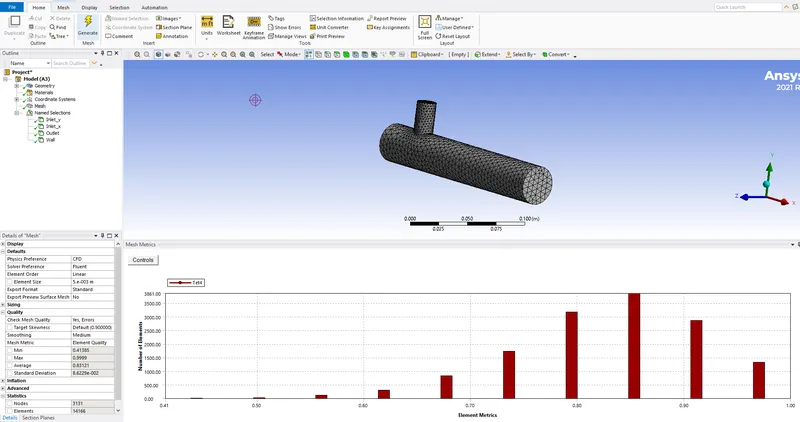
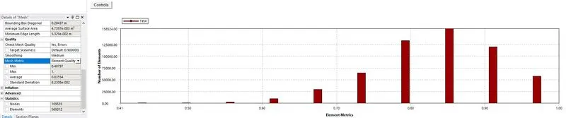
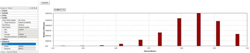
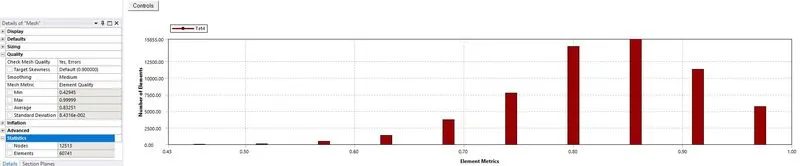
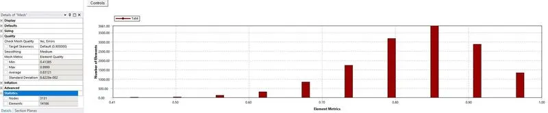
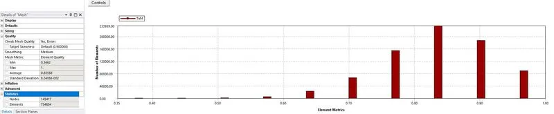
We change the element size to 0.005 as shown in the above image also we see thw element quality graph as show in the above image. The mesh is updated after clicking the updarte and the window is closed.
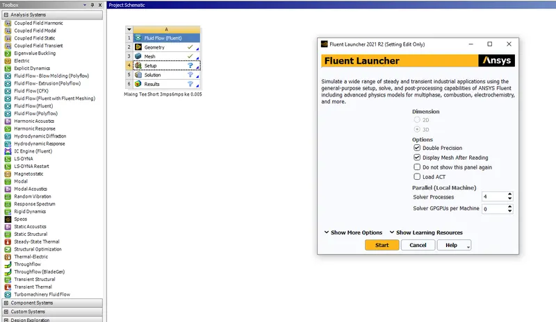
On clicking the Setup, Fluent Launcher Window Pops up, select as shown in the above image.
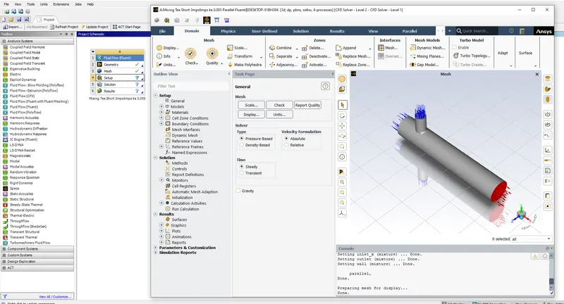
The Ansys Fluent window pops up as shown in the above image. In the Solver we select Type as Pressure based, Velocity formulation as Absolute and Time as Steady state.
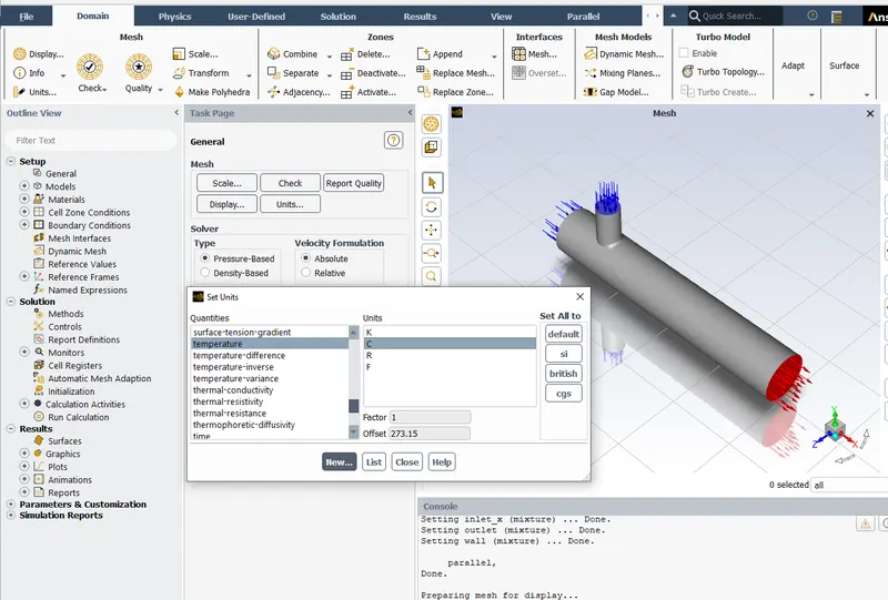
The units can be changed by clicking the Units under Mesh in Domain as shown in the above image.
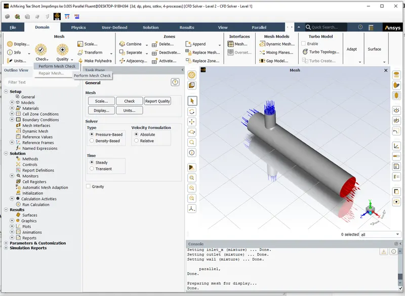
The mesh check is performed using Perform Mesh Check in Check under Mesh in Domain as shown in the above image.
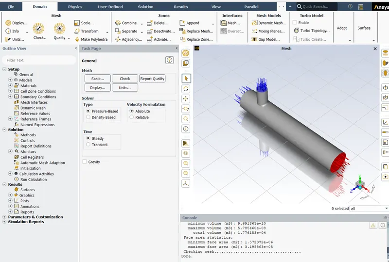
Mesh checking is done and no errors were encountered. Refer Console as shown int the above image for Mesh details checked.
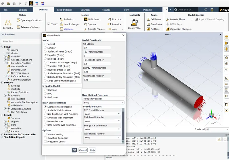
Now I select the Energy under Models since we are interested in temperature variance during simulation.
For viscous model I select the options as shown in the above image.
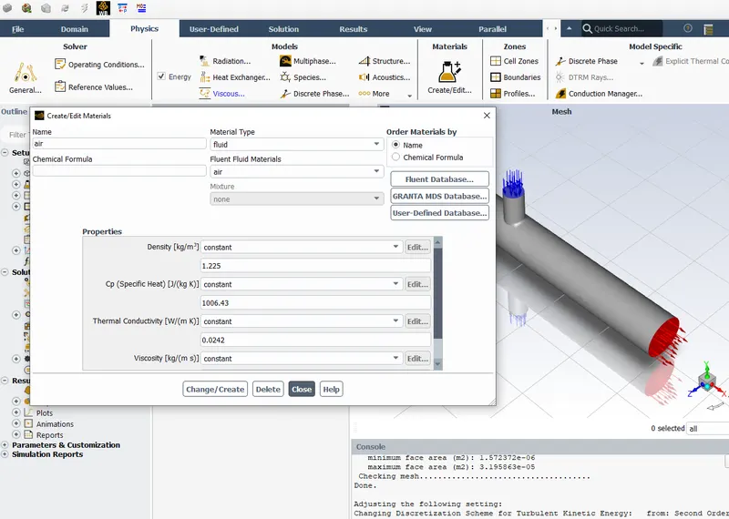
The type of fluid involved in the process can be selected/edited using the method as shown in the above image.
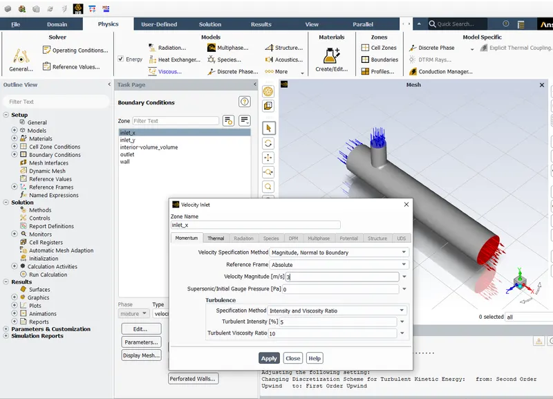
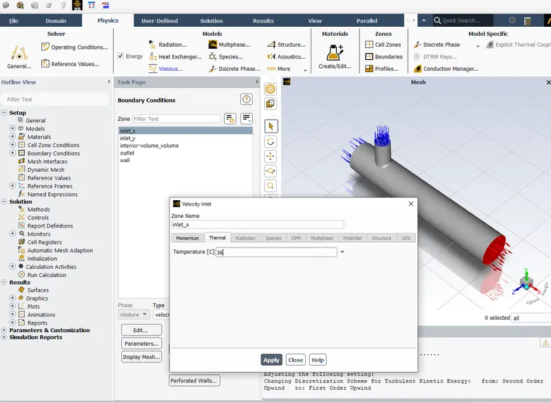
The boundary conditions can be defined as shown in the above two image.
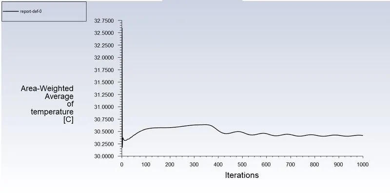
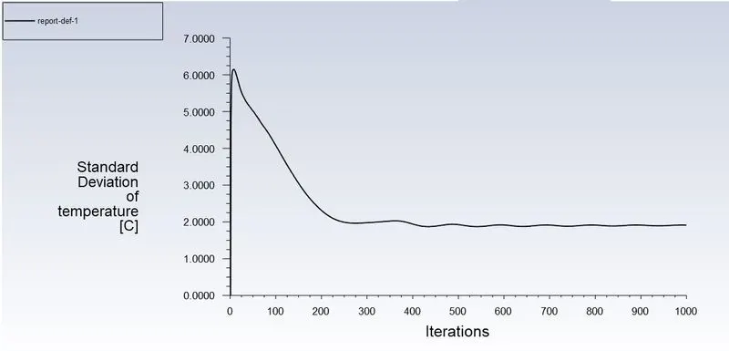
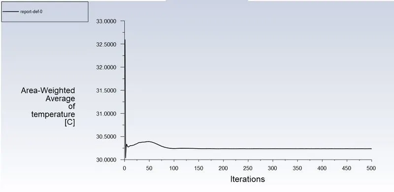
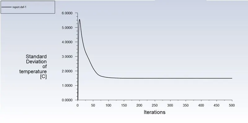
Definitions for Areaweighted average and standard deviation is done using Definitions under Reports.
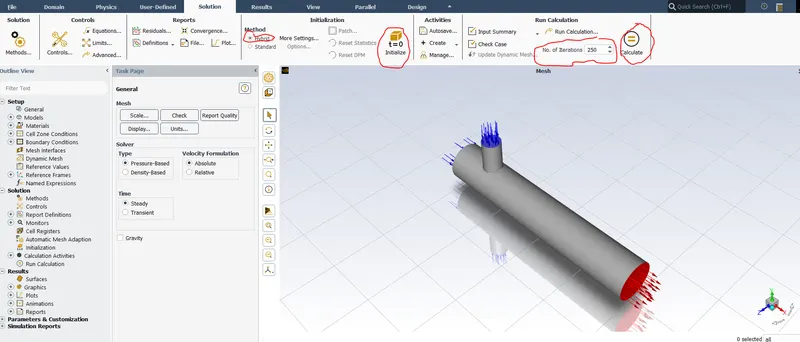
Initialization is done using Hybrid option, Number of iterations is set to 250 and calculate is option is clicked as shown in the above image.
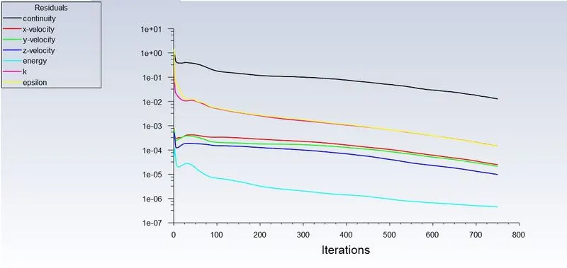
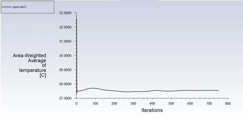
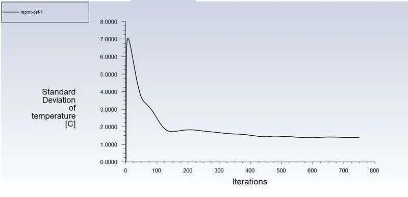
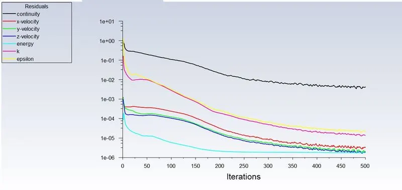
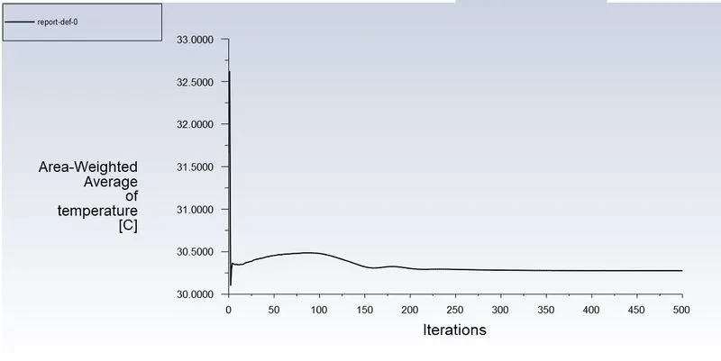
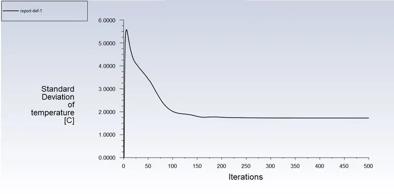
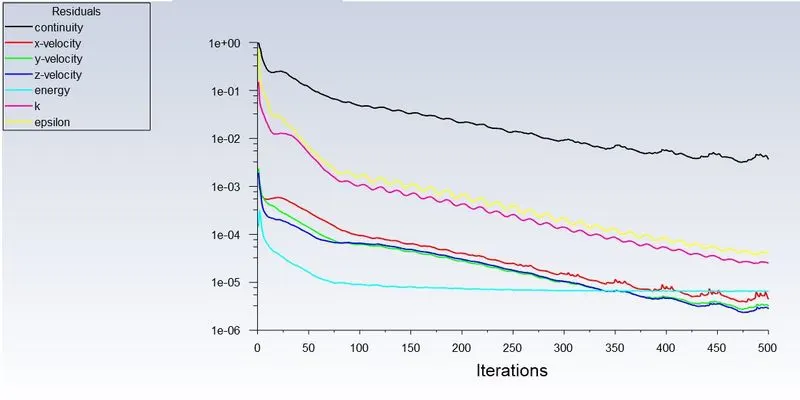
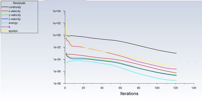
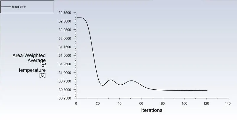
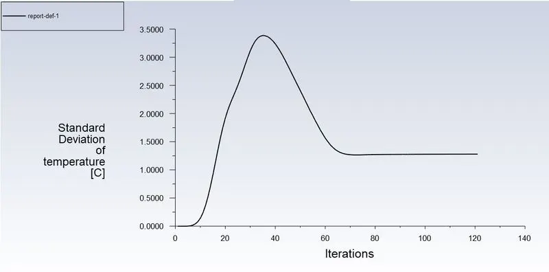
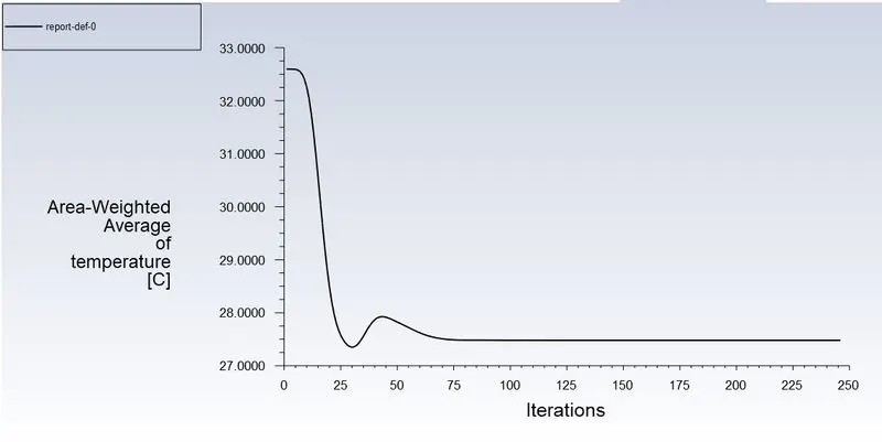
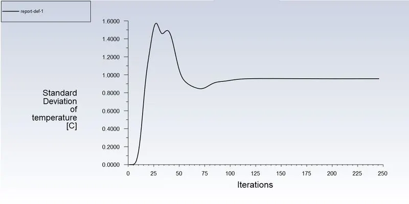
The residuals, area weighted average plot for temperature and standard deviation of temperature for individual cases has been inserted below.
Using CFD Post, temperature and velocity contours generated has been inserted below.
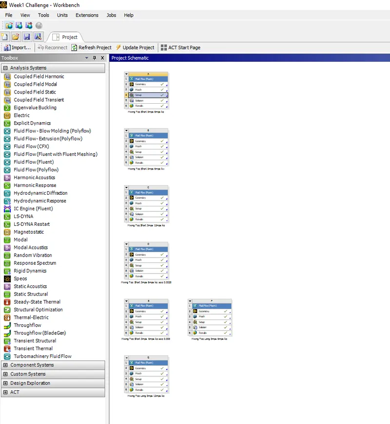
CASE 1 : Mixing Tee Short, Hot Inlet Velocity 3m/s, Momentum Ratio 2, k-epsilon, Mesh size 0.001m
MESHING
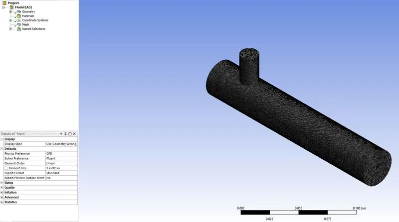
ELEMENT QUALITY GRAPH
RESIDUALS PLOT
AREA WEIGHTED AVERAGE PLOT OF TEMPERATURE
STANDARD DEVIATION PLOT OF TEMPERATURE
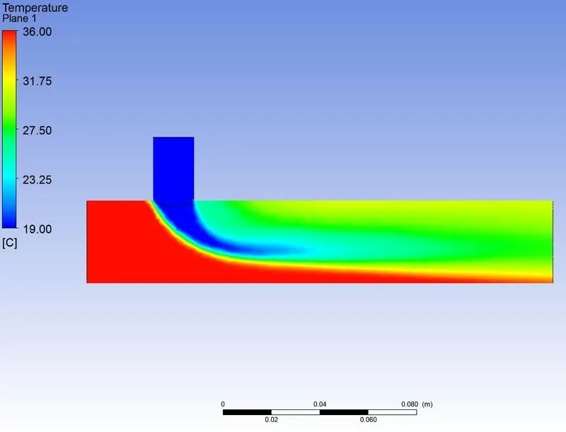
TEMPERATURE CONTOUR PLOT ALONG THE PIPE
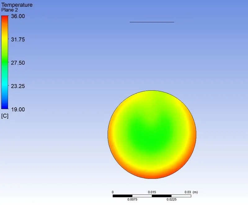
TEMPERATURE CONTOUR PLOT ACROSS THE PIPE NEAR OUTLET
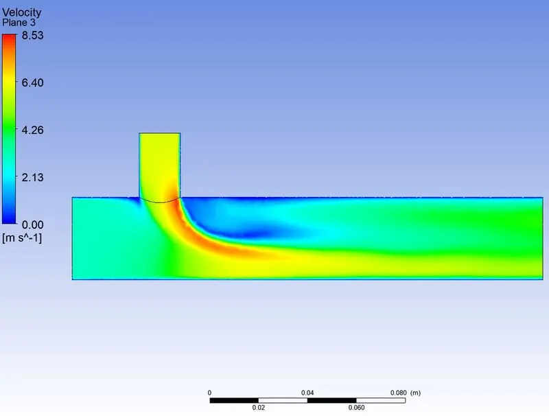
VELOCITY CONTOUR PLOT ALONG THE PIPE
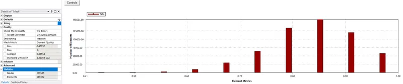
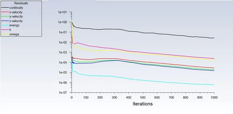
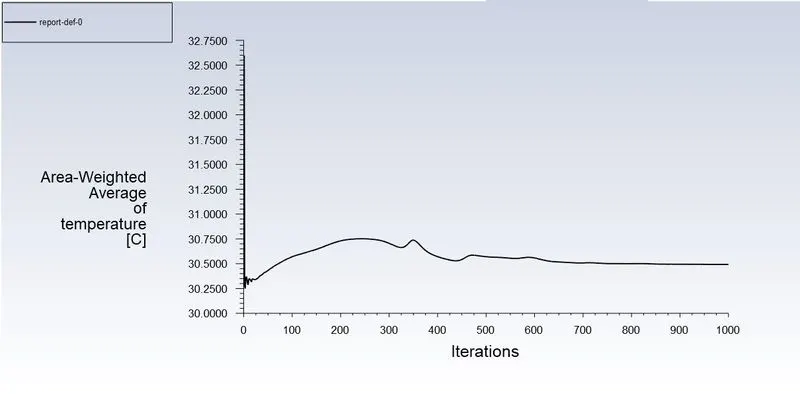
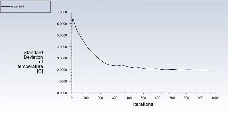
CASE 1A : Mixing Tee Short, Hot Inlet Velocity 3m/s, Momentum Ratio 2, k-omega, Mesh size 0.001m
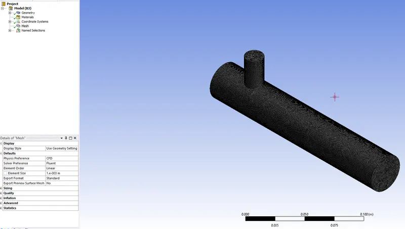
MESHING
ELEMENT QUALITY GRAPH
RESIDUALS PLOT
AREA WEIGHTED AVERAGE PLOT OF TEMPERATURE
STANDARD DEVIATION PLOT OF TEMPERATURE
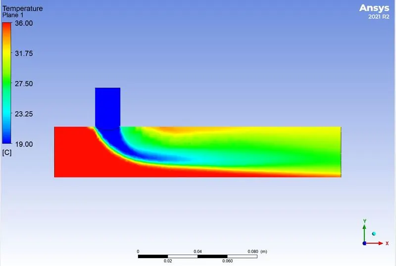
TEMPERATURE CONTOUR PLOT ALONG THE PIPE
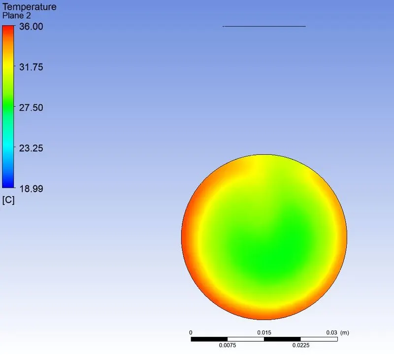
TEMPERATURE CONTOUR PLOT ACROSS THE PIPE NEAR OUTLET
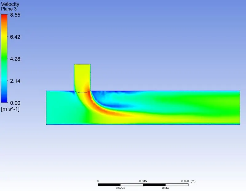
VELOCITY CONTOUR PLOT ALONG THE PIPE
CASE 1B : Mixing Tee Short, Hot Inlet Velocity 3m/s, Momentum Ratio 4, k-epsilon, Mesh size 0.001m
MESHING
ELEMENT QUALITY GRAPH
RESIDUALS PLOT
AREA WEIGHTED AVERAGE PLOT OF TEMPERATURE
STANDARD DEVIATION PLOT OF TEMPERATURE
TEMPERATURE CONTOUR PLOT ALONG THE PIPE
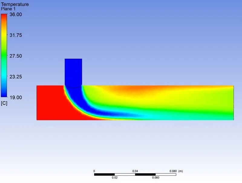
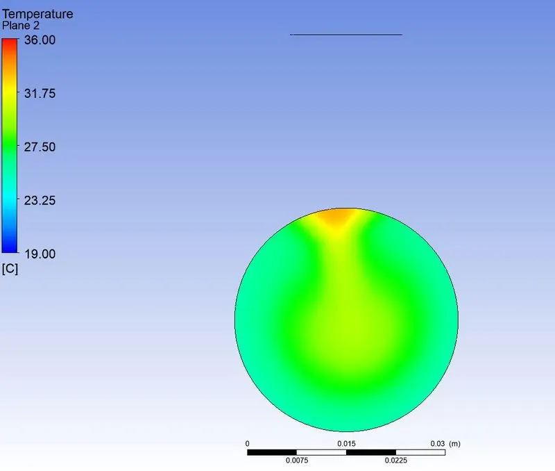
TEMPERATURE CONTOUR PLOT ACROSS THE PIPE NEAR OUTLET
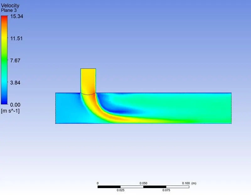
VELOCITY CONTOUR PLOT ALONG THE PIPE
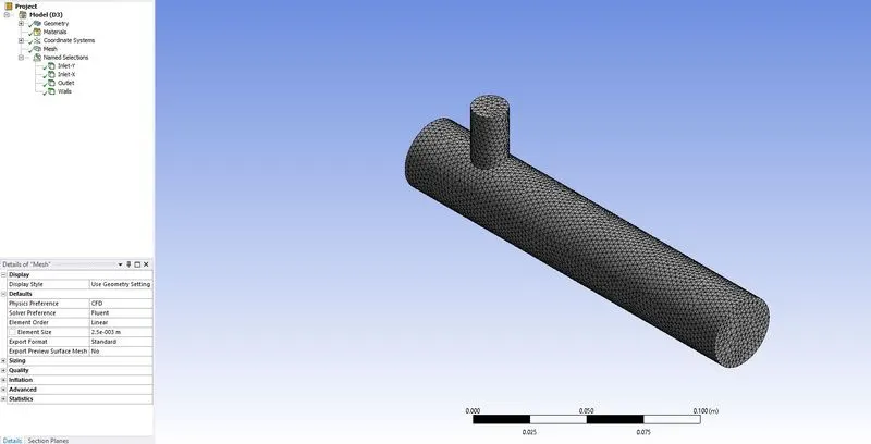
CASE 1C : Mixing Tee Short, Hot Inlet Velocity 3m/s, Momentum Ratio 2, k-epsilon, Mesh size 0.0025m
MESHING
ELEMENT QUALITY GRAPH
RESIDUALS PLOT
AREA WEIGHTED AVERAGE PLOT OF TEMPERATURE
STANDARD DEVIATION PLOT OF TEMPERATURE
TEMPERATURE CONTOUR PLOT ALONG THE PIPE
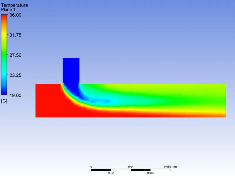
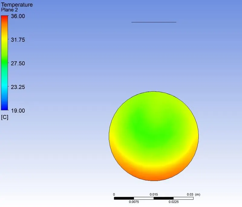
TEMPERATURE CONTOUR PLOT ACROSS THE PIPE NEAR OUTLET
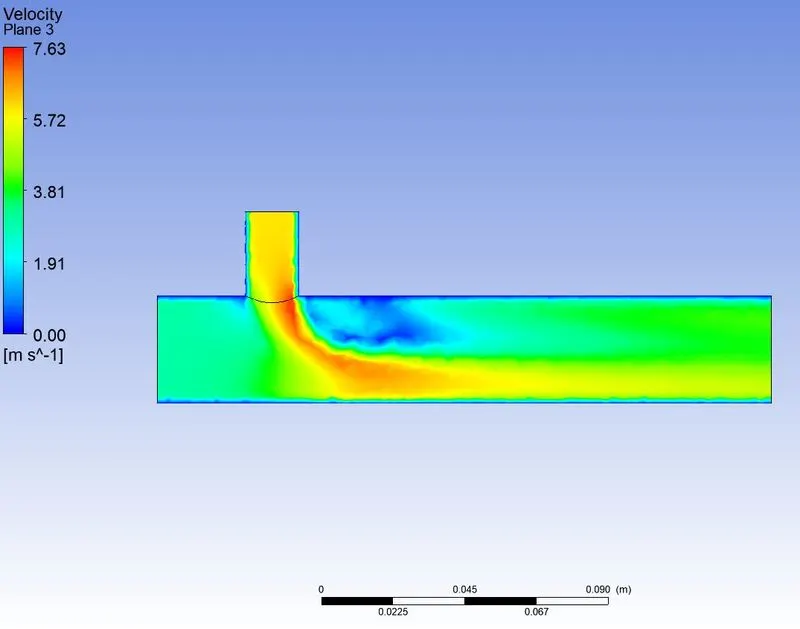
VELOCITY CONTOUR PLOT ALONG THE PIPE
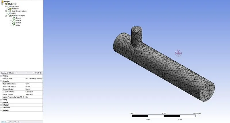
CASE 1D : Mixing Tee Short, Hot Inlet Velocity 3m/s, Momentum Ratio 2, k-epsilon, Mesh size 0.005m
MESHING
ELEMENT QUALITY GRAPH
RESIDUALS PLOT
AREA WEIGHTED AVERAGE PLOT OF TEMPERATURE
STANDARD DEVIATION PLOT OF TEMPERATURE
TEMPERATURE CONTOUR PLOT ALONG THE PIPE
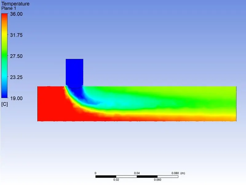
TEMPERATURE CONTOUR PLOT ACROSS THE PIPE NEAR OUTLET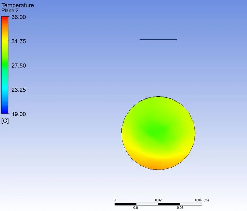
VELOCITY CONTOUR PLOT ALONG THE PIPE
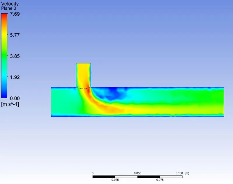
CASE 2 : Mixing Tee Long, Hot Inlet Velocity 3m/s, Momentum Ratio 2, k-epsilon, Mesh size 0.001m
MESHING
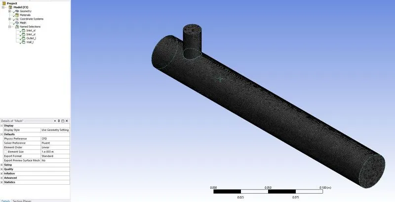
ELEMENT QUALITY GRAPH
RESIDUALS PLOT
AREA WEIGHTED AVERAGE PLOT OF TEMPERATURE
STANDARD DEVIATION PLOT OF TEMPERATURE
TEMPERATURE CONTOUR PLOT ALONG THE PIPE
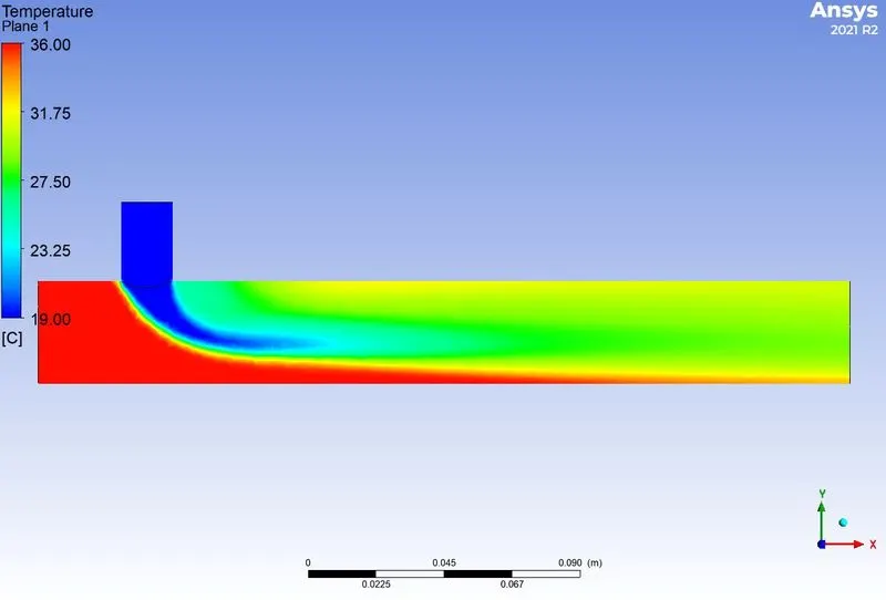
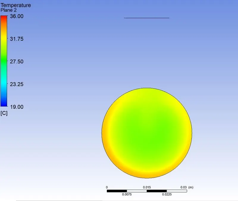
TEMPERATURE CONTOUR PLOT ACROSS THE PIPE NEAR OUTLET
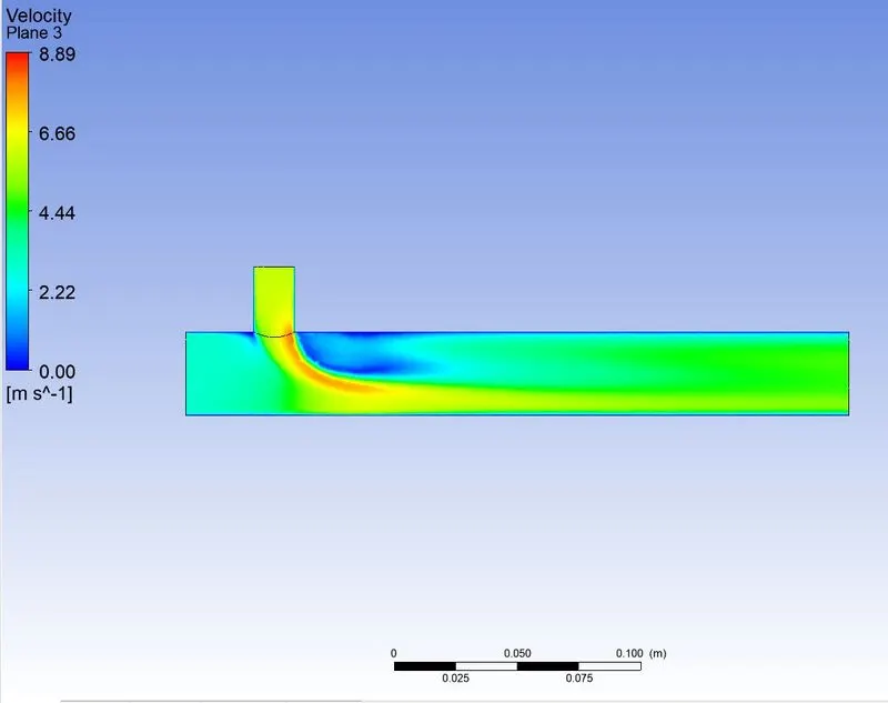
VELOCITY CONTOUR PLOT ALONG THE PIPE
CASE 2A : Mixing Tee Long, Hot Inlet Velocity 3m/s, Momentum Ratio 4, k-epsilon, Mesh size 0.001m
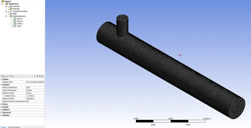
MESHING
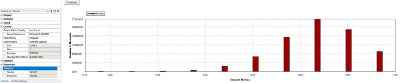
ELEMENT QUALITY GRAPH
RESIDUALS PLOT
AREA WEIGHTED AVERAGE PLOT OF TEMPERATURE
STANDARD DEVIATION PLOT OF TEMPERATURE
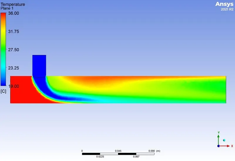
TEMPERATURE CONTOUR PLOT ALONG THE PIPE
TEMPERATURE CONTOUR PLOT ACROSS THE PIPE NEAR OUTLET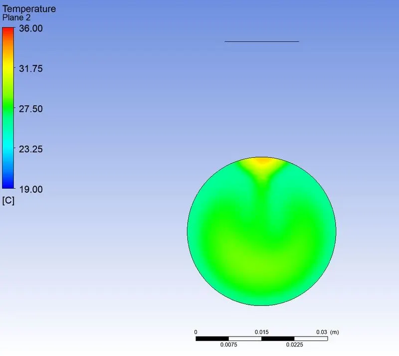
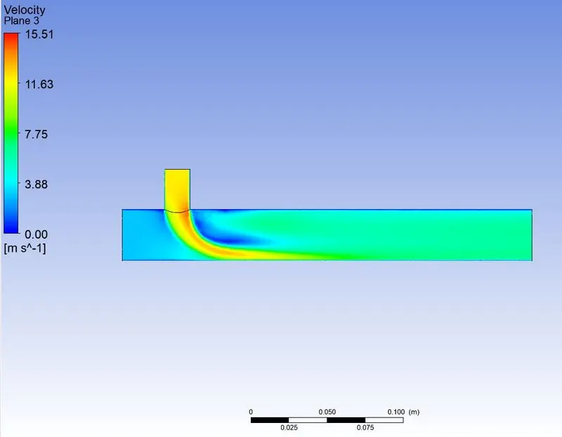
VELOCITY CONTOUR PLOT ALONG THE PIPE
CONCLUSION:
- The flow in a mixing tee geometry was simulated successfully for both the models (Mixing Tee Long & Mixing Tee Short) using Ansys Fluent Software.
- k-epsilon models predict flow virtually far from the boundaries (wall), and the k-omega model predicts near the wall. In this case, we need a flow simulation turbulent model far from the wall, therefore, the k-epsilon method is used.
- Solving the first simulation on the fluid domain using coarse mesh gives an initial overview of the analysis which converges results fast. As the element number increases the convergence time also increases. Therefore, after obtaining the rough results using coarse mesh simulation successfully we can improve mesh quality and get final accurate results doing this saves a lot of time which is also extremely helpful for the mesh independence tests.
- To get better mixing at the outlet, high velocity of cold fluid inlet flow is very effective. Therefore, a higher momentum ratio gives better mixing of hot and cold fluid streams at the outlet.
- In the above cases, it is very important to use a short mixing tee with a momentum ratio of 4 to get precise results.
- One can consider the diffusion of flow along the length of the mixing tee, a long mixing tee with momentum will be the greater option.