Week 1- Mixing Tee

Aim:- set up steady-state simulations to compare the mixing effectiveness when hot inlet temperature is 36⁰C & the Cold inlet is at 19⁰C.

Use the k-epsilon model.

1. Case 1
   • Short mixing tee with a hot inlet velocity of 3m/s.
   • Momentum ratio of 2, 4.
2. Case 2
   • Long mixing tee with a hot inlet velocity of 3m/s.
   • Momentum ratio of 2, 4.

Momentum ratio = velocity at cold inlet / velocity at hot inlet

In a table, compare the following values from the 2 cases.

1. Cell count
2. Average outlet temperature
3. Number of iterations for convergence

Theroy:- Computational fluid dynamics or CFD is the analysis of systems involving fluid flow, heat transfer and associated phenomena such as chemical reactions by means of computer-based simulation.

Practical application in current scenario

• aerodynamics of aircraft and vehicles: lift and drag
• hydrodynamics of ships
• power plant: combustion in internal combustion engines and gas
turbines
• turbomachinery: flows inside rotating passages, diffusers etc.
• electrical and electronic engineering: cooling of equipment including
microcircuits
• chemical process engineering: mixing and separation, polymer moulding
• external and internal environment of buildings: wind loading and
heating/ventilation
• marine engineering: loads on off-shore structures
• environmental engineering: distribution of pollutants and effluents
• hydrology and oceanography: flows in rivers, estuaries, oceans
• meteorology: weather prediction
• biomedical engineering: blood flows through arteries and veins

CFD Work Flow:- CFD codes are structured around the numerical algorithms that can tackle fluid flow problems. In order to provide easy access to their solving power all commercial CFD packages include sophisticated user interfaces to input problem parameters and to examine the results

Its threee step process
(i) a pre-processor

involves defination of geometry, grid generation, selection of phenomenon that need to model

(ii) a solver

intergration of governing equation, discretisation and solution

(iii) a post-processor

ploting of contour, graphs and making movies.

In solving fluid flow problems we need to be aware that the underlyingphysics is complex and the results generated by a CFD code are at best asgood as the physics (and chemistry) embedded in it and at worst as good asits operator with CFD

Therory About Tee:-

Tee is a combination of pipe formed when the are alligned or joined in such a way that they are are 90 degree to each other. In this type of arrangment one fluid which is hot fluid passing in straight direction where as cold fluid enter in perpedicular direction to the hold fluid. We are intrested in knowing some parameters like average temp, effectiveness, std deviation of temprature, velocity profile other things. The flow arrangement we are dealing in this situation is side tee, there are different tee arrangment present like opposed tee model and multiple tee model, which have different application as per industrial point of view.

This type of tee arrangment i.e. side tee arrangment is used in different industries like HVAC and thermal power plant. before designing the flow system we need to consider and analyse the operating temprature and velocity of the working fluid we are intested in.

Solving and Modeling Approch:-

There are no way present to understand and analyse the effeciveness of the mixiing tee model.

1. analytical approch

2. simulation approch

3. experimental approch

using analytical approch and experimental approch is time consuming and high cost senario. this could be eliminated by using simulation approch in which we can analyse the system with the actual codition we are intrested in.

To do this we are using ansys fluent solver

we are using fluid flow analysis using Fluent solver because we are interested in the total effectiveness of the fluid in the mechnical tee model, here we are using two different models to analyse the effectiveness of the mixing of fluid.

Mesh length choose as 3mm

Approch we are using.

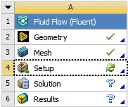
1. We need to open Ansys workbench

2. Choose the Appropiate Solver

3. Assign Appropiate name

4. Choose geometry and select new spaceclaim model.

5. Load the appropiate file

6. Implement the geometrical operation

7. Apply the mesh and provide name selection

8. Choose setup, select the appropiate model

9. Initalisation and running the simulation

10. Result making i.e. countour plots graphs

Preprocessing and solver settings:-

1. Opening Ansys workbench

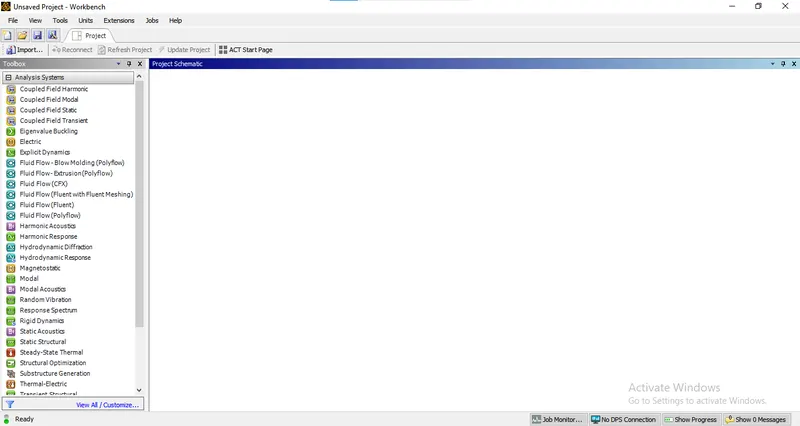
2. Choose the Appropiate Solver

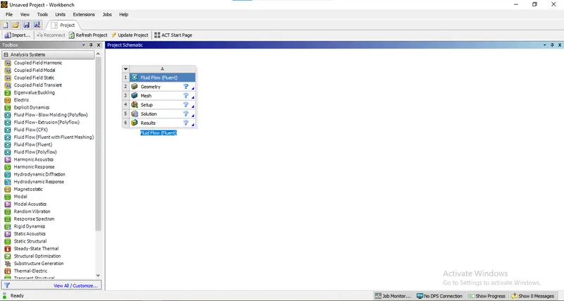
3. Assign Appropiate name

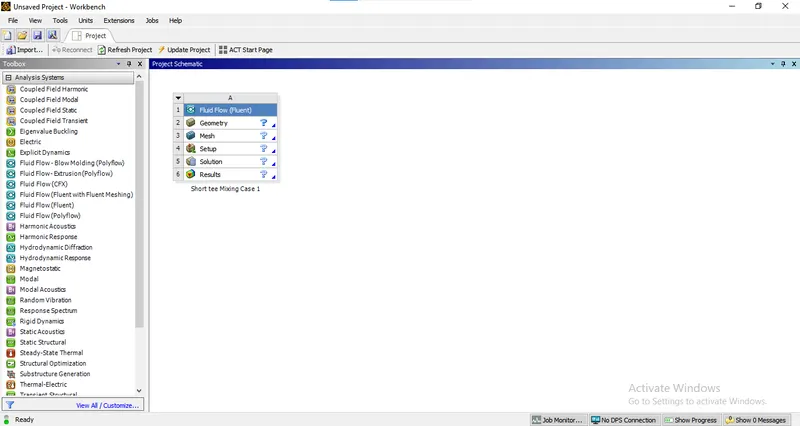
5. Choose geometry do to geometrical operation

choose the geometry>right click and choose spaceclaim>choose the file

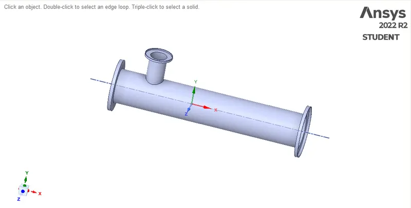
6. Implementing the geometric operation

1. go to preapre>select volume extract>select edge option

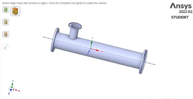
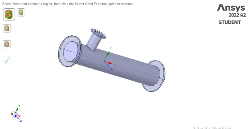
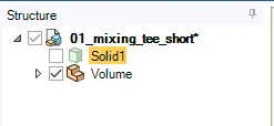
2. right click on the solid and supress for physics

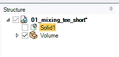
Close the space claim window.

7. Applying the mesh

go to the mesh

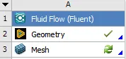
right click and edit

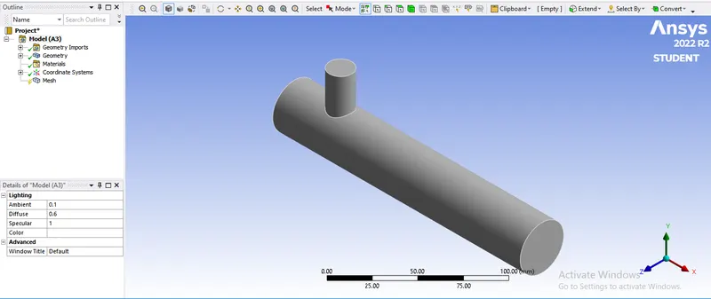
click on mesh>check the appropiate mesh length we are choosing 3 mm.

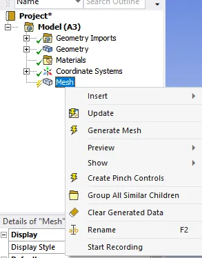
click generate option.

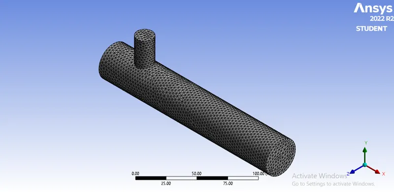
Now we provide the name selection.

go to face selection>select the face>press N or right click>enter an appropiate name

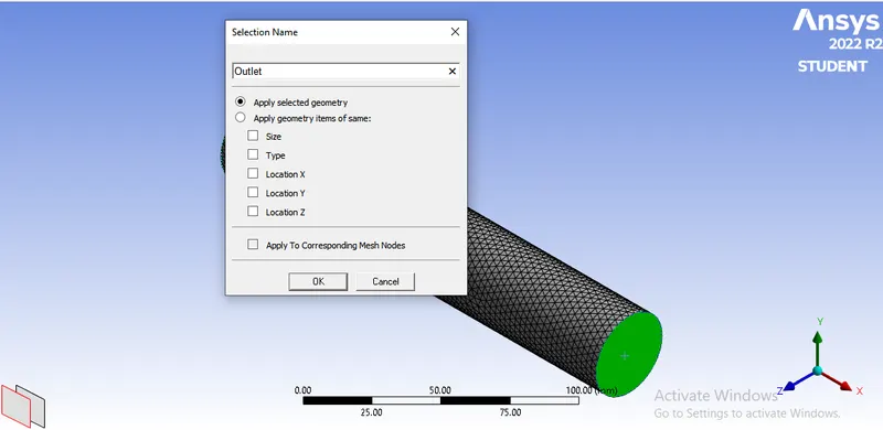
in similar manner we assign the name

input X

input Y

Wall

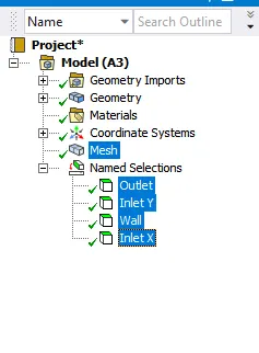
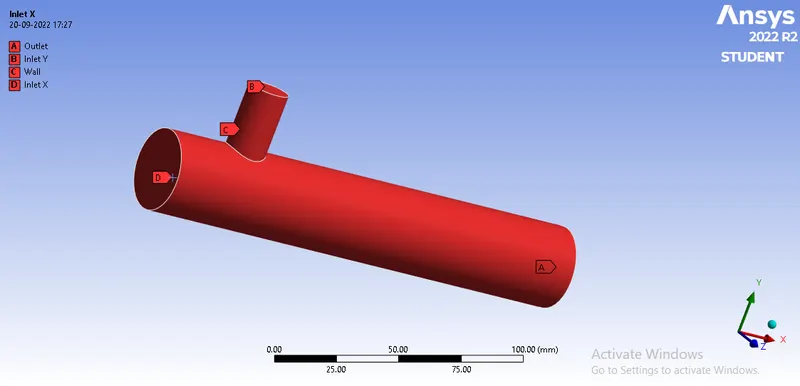
update the mesh by clicking the right mouse button on mesh and update.

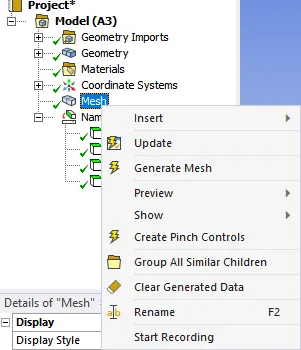
Close the Mesh window.

8. Choose setup

1. checking for the mesh.

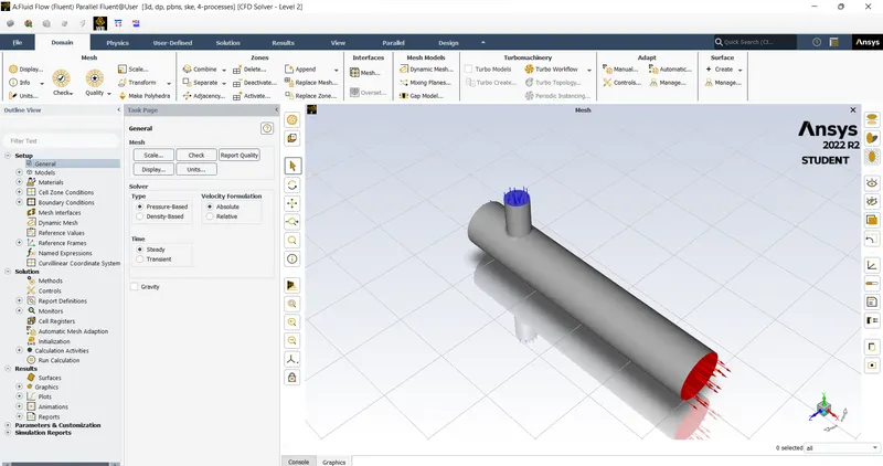
make sure we chooses the solver type as pressure- based model and velocilty formulation as absolute time state as steady.

if mach no<.3 pressure based model

if mach no>.3 density based model

task page>general>mesh>check

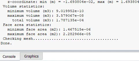
mesh checking is done.

2. Go to physics and enable the energy equation becuase we are instrested in knowing the temprature of the outlet and choose k-epsilone model

for turbluent analysis we use k-eplison and k-omega model, both used 2 equation to solve the problem.

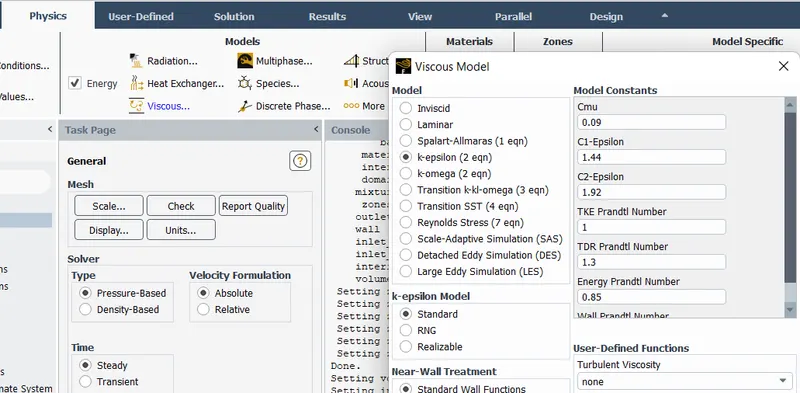
3. we can change the working material and cell zone condition, but in this case we choose air as working medium.

4. apply the boundary condition.

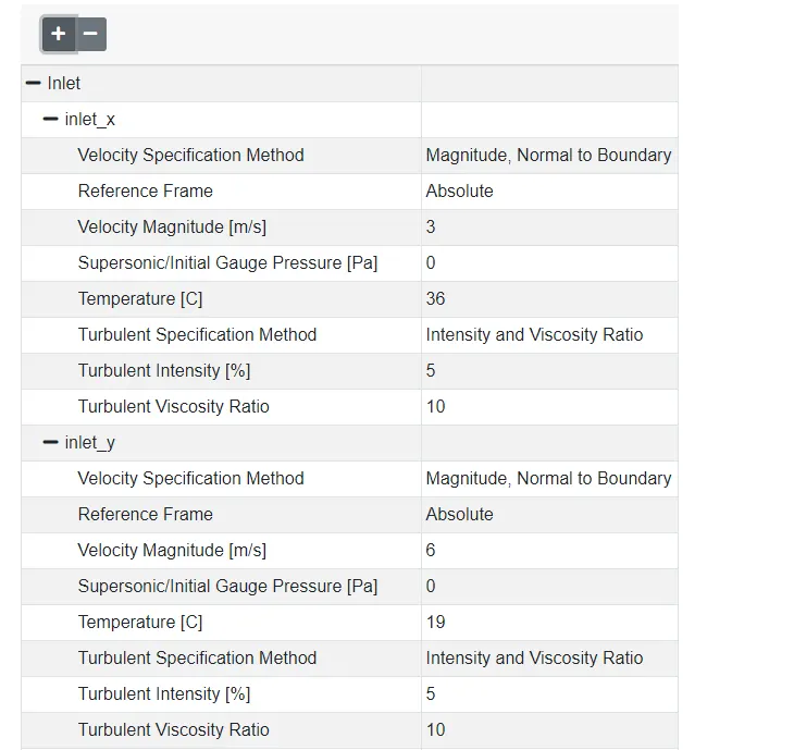
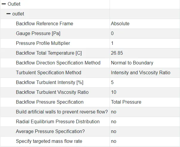
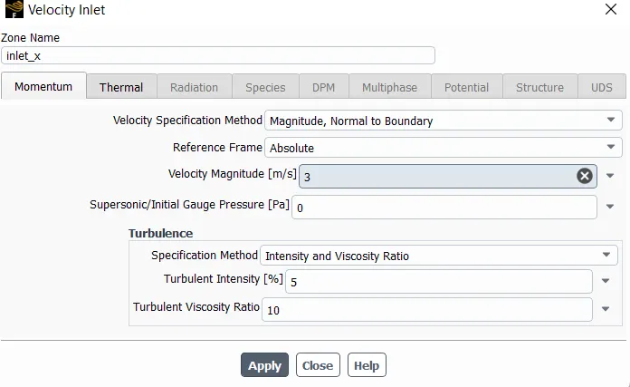
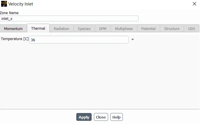
go to physics>zone>boundary coondition

case 01

• hot inlet velocity of 3m/s. Temphot =36 C & Tempcold=19 C
• Momentum ratio of 2.( Vhot = 3 m/s, VCold = 6 m/s)

case 02

• hot inlet velocity of 3m/s. Temphot =36 C & Tempcold=19 C
• Momentum ratio of 2.( Vhot = 3 m/s, VCold = 12 m/s)

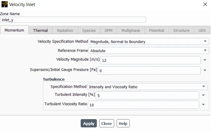
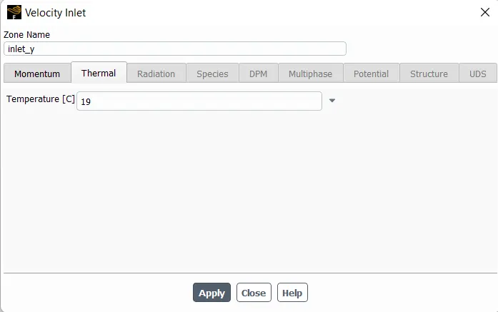
in similar manner we apply to inlet Y

5. Select solution tab>defination>choose new

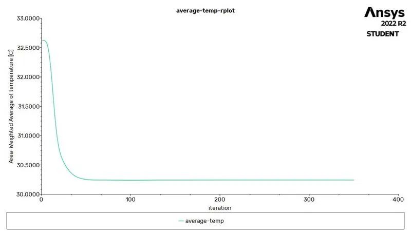
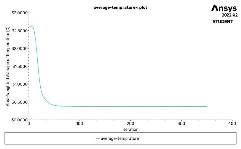
1. average temp

choose new>surface report>area weighted average

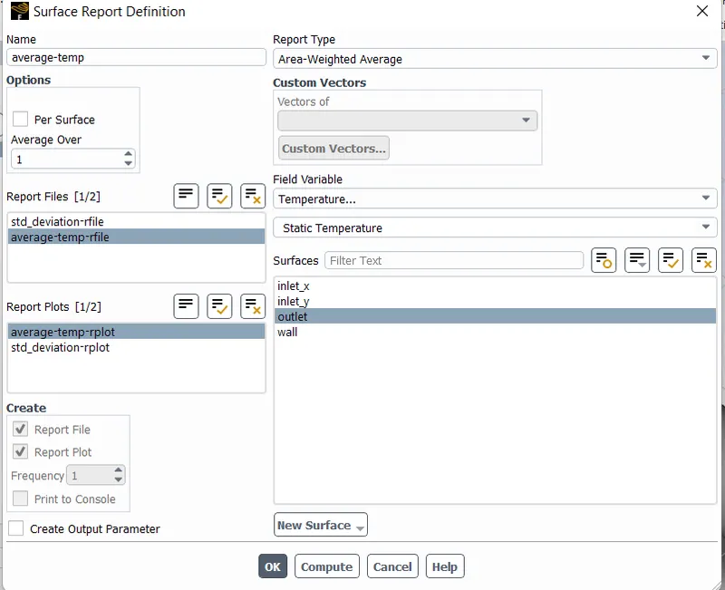
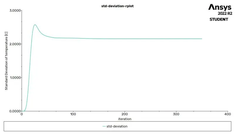
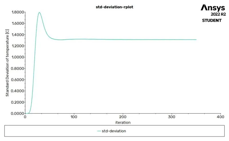
2. Std devation

choose new>surface report>standard deviation

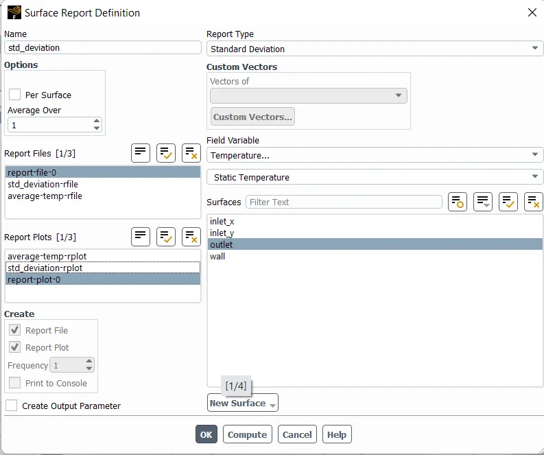
9. Now we initialise the program.

solution tap>initialization

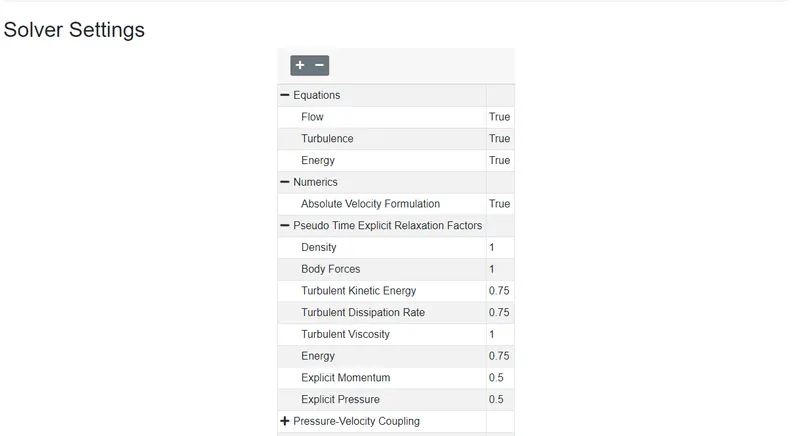
10. Solver settings.

10. Repeat the same step for

case 02 short tee

case 01 long tee

case 02 long tee

11. Results

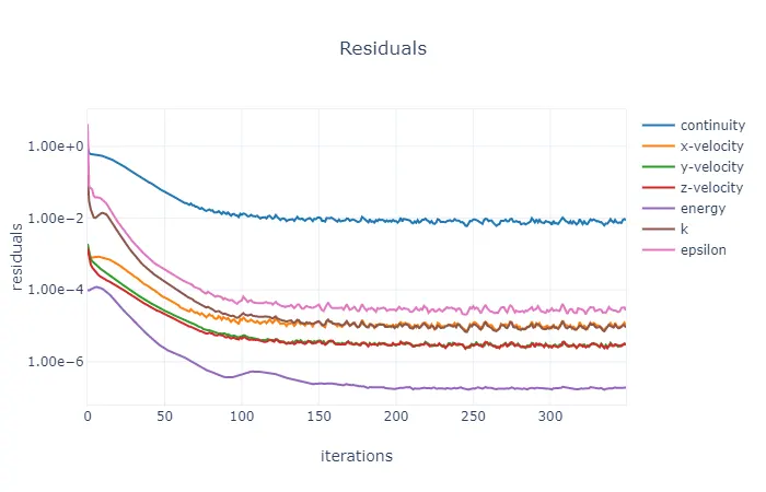
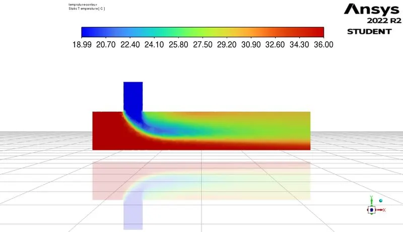
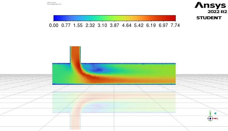
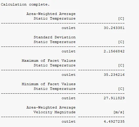
case 01 short tee

MR 2

case 02 short tee

MR 4

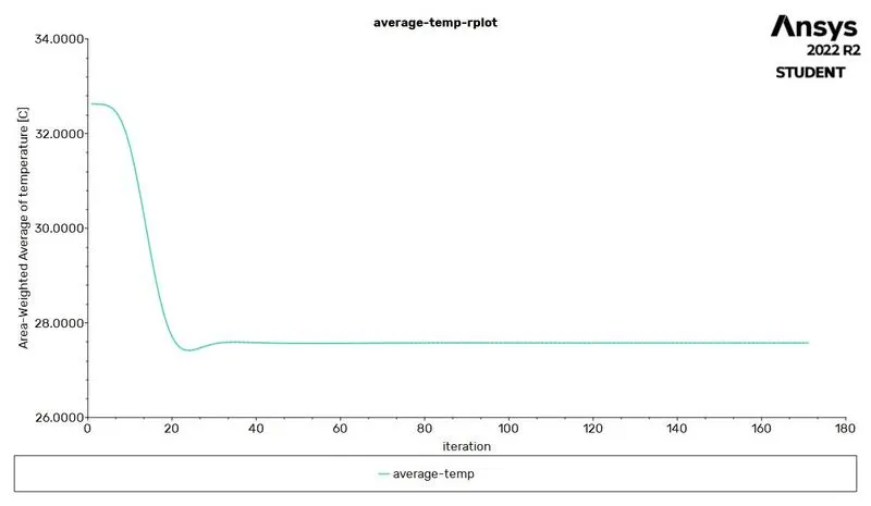
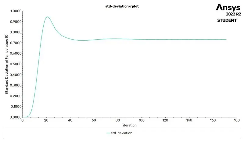
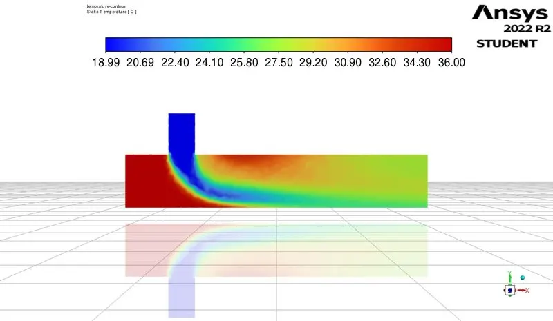
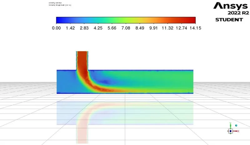
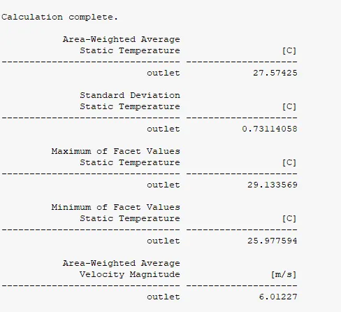
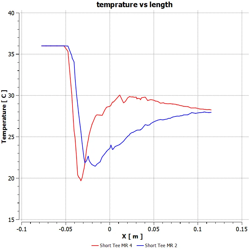
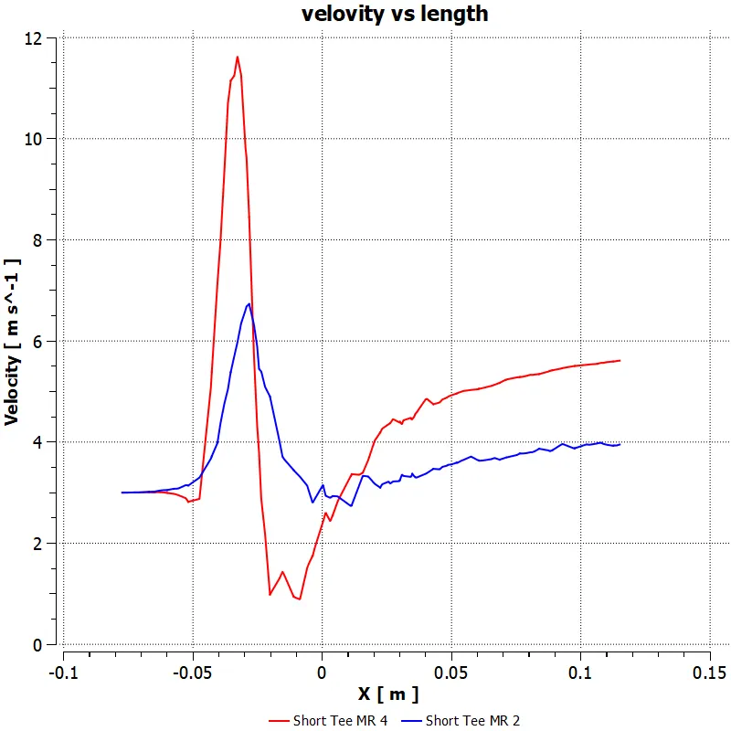
comparision graphs mr 2 vs mr 4 short tee

temprature vs length

Conclusion

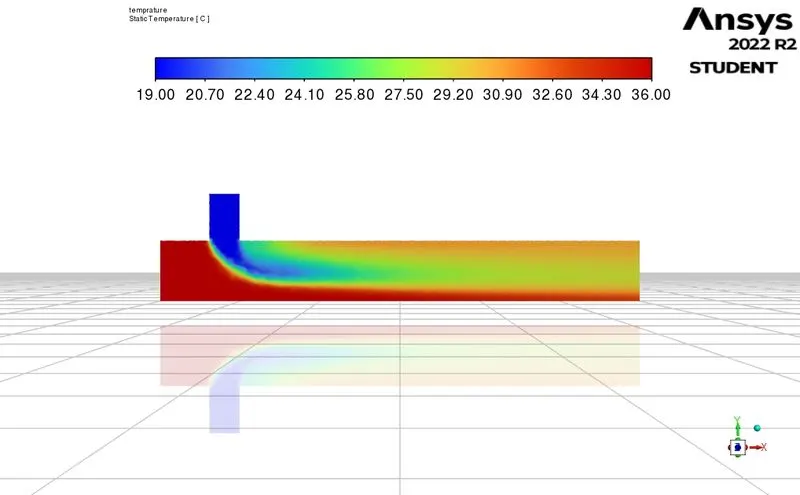
1. in case of short tee MR2 vs MR4 temprature the final temprature at the outlet is nearby same, there is a sudden change in temprature becuse cold fluid enter in the system.

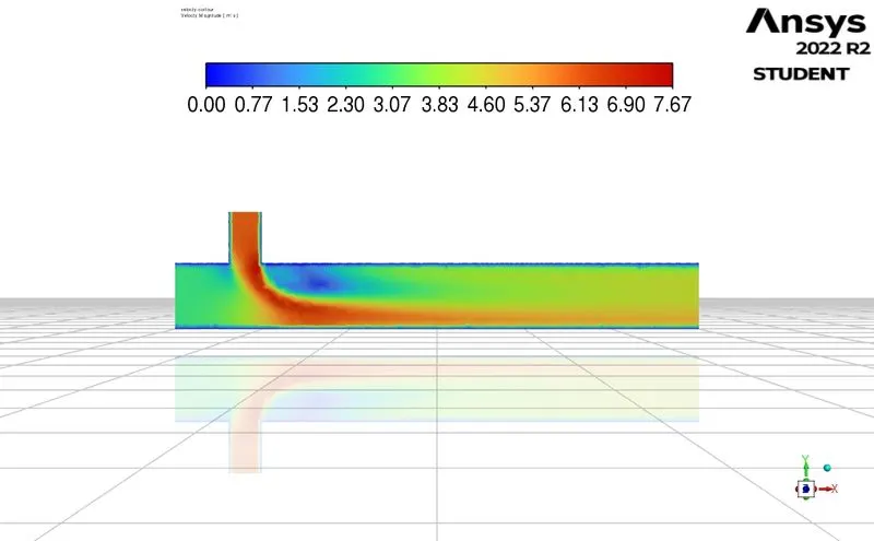
2. in case of short tee MR2 vs MR4 velocity there is sudden rise in velocity in case of mr4 becuase cold fluid velocity is about 12m/s and in case of mr2 velocity of cold fluid is 6m/s

3. effectiveness is better in mr4 as compared to mr2, low std deviation indicates good effectiveness

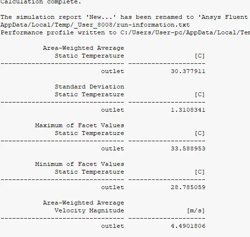
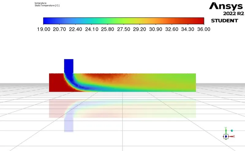
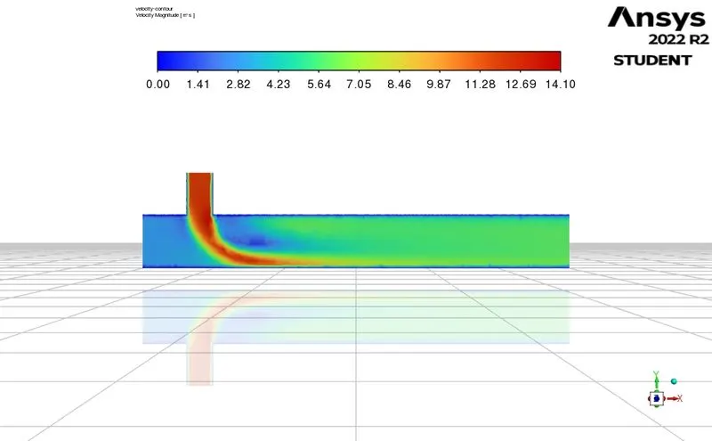
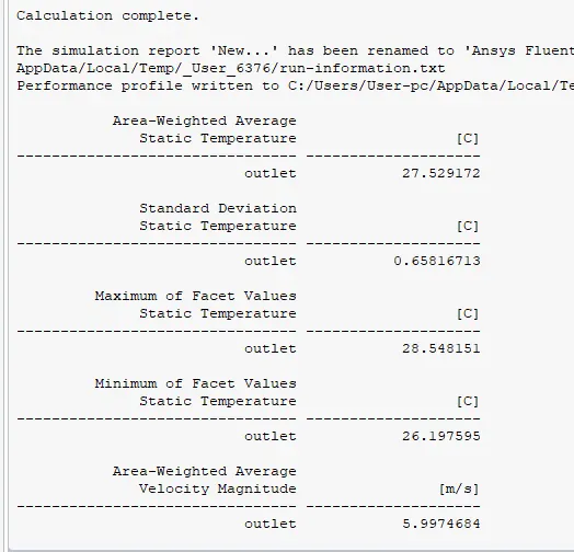
case 01 long tee

MR 2

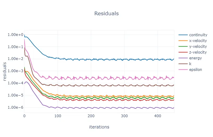
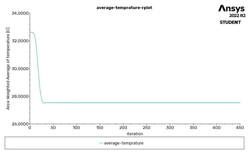
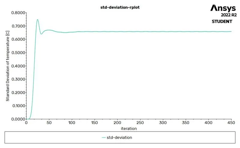
case 02 long tee

MR 4

comparision graphs mr 2 vs mr 4 short tee

temprature vs length

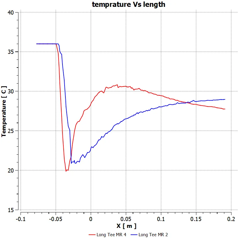
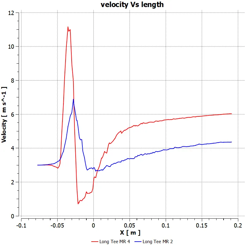
1. in case of short tee MR2 vs MR4 temprature the final temprature at the outlet is nearby same, there is a sudden change in temprature becuse cold fluid enter in the system.and we get low temprature at outlet when we are increasing the velocity of cold fluid

2. in case of short tee MR2 vs MR4 velocity there is sudden rise in velocity in case of mr4 becuase cold fluid velocity is about 12m/s and in case of mr2 velocity of cold fluid is 6m/s there is no such changed observed in velocity

3. effectiveness is better in mr4 as compared to mr2, low std deviation indicates good effectiveness

Conclusion

from the results we obtained from all 4 cases and its comparison, we can say that case 2 is better among the 4. Let us see the analysis data from the simulation as well in the below tabulation for mesh element size 3mm and k epsilon model.

Parameter		Short Tee		Long Tee
		MR 2	MR 4	MR 2	MR 4
Average Temperatur	Simulation	30.29	27.58	30.35	27.52
	Numerical	30.24	27.57	30.37	27.52
	% Error	5%	1%	-2%	0%
Average Velocity m/s		4.49	6.01	4.49	5.99
Standard Deviation Of Temprature		2.15	0.73	1.31	0.65

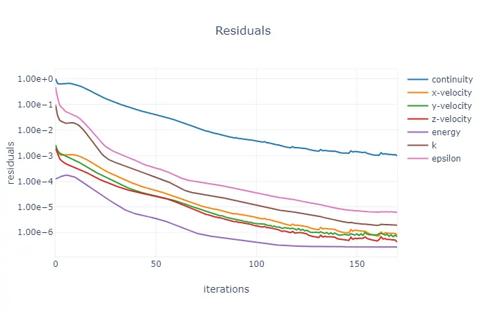
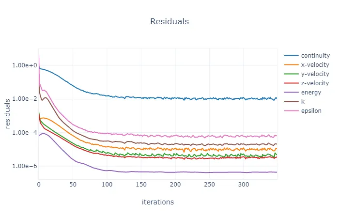
the only conversed solution we get is for short tee MR 4

Final Conclusion:-

1. increase in length of tee reduce the average velocity at outlet

2. final result will be affected by the cold fluid inlet velocity and temp

3. sudden decrement in the temprature when cold fluid mix with hold fluid

4. as the length of tee increases greater will be the effectivenesss

5. velocity is very high when two fluid mix which create a flow sepration and vertex or negative pressure reason

6. short tee case two is better we can conversed solution at 147iteration, we can improve the effectiveness just by modifying the inlet angle.

Note:- No snippets is used.