Week 1- Mixing Tee
Notice: - After the analysis, the size of the file is more, but in the challenge submission time it is not supported because of its large so I am sharing the google drive link please download from the link.
Link: https://drive.google.com/file/d/1z4wRSrWu-h7qFgqIDP9XZvAdbRZ2ShyE/view?usp=drivesdk
Introduction
In the turbulent mixing tee model, we use two fluid which has two properties in the different inlet. The fluids are in different temperatures and different velocities which are playing an important role in the T-junction of the model. Temperature fluctuation is happening in the mixing tee model with respect to the distance covered by the mixing air. We use here two types of models where one has a shorter length and another one has a longer length. We are using Ansys fluent for the CFD simulation of the turbulence mixing model. We are considering some models to define the appropriate values of the mixing air.
In our practical life, we use air conditioning systems for the human body’s comfort, but this comfort temperature will be different when the season will change. In this condition air conditioner gives a lower temperature air where the human body needs more temperature in the atmosphere for this condition, we use the atmospheric temperature with some velocity to increase the temperature of the air, for this condition we use a mixing tee. This mixing of air creates turbulence conditions which fluctuate the temperature in the wall and outlet. In the Ansys fluent mesh parameter and solving the problem by CFD simulation and giving a detailed description of the result, we can use these data to compare with the experimental data.
Solving & modelling approach
Here we consider two models as compared to the length of the pipe one is a shorter length the other is a longer length where other dimensions are the same. In this CFD simulation of turbulence mixing tee, we are considering two models for the solution to the problem, one is k-epsilon with RANS (Reynolds-Average Navier-stokes equation) and another one is the k-omega SST model. We are using these two models of the equation for solving the problem. The temperature near the wall is fluctuating after the mixing of hot air and cold air with some velocity. We can use the temperature and velocity counter-plot for the detailed analysis of the problem. When seen in the counter-plot diagram of temperature, after mixing the two-temperature air temperature will start fluctuating, this temperature diagram also depends upon the mesh element size.
In the temperature counter plot diagram also can see the velocity profile in the different positions, in the near the wall the velocity will be zero because of the no-slip condition, here the velocity profile will fluctuate as compared to the element mesh size. In the result after the simulation, some iterations will take to converge the solution. For the converge solution we use basically the discretization methods. These discretization methods are basically the computer language which use to solve the partial differential equations.
Discretization methods are 3 types
- Finite element method
- Finite difference method
- Finite volume method
We use these methods for structural analysis, conservation and for hyperbolic functions. For computational fluid dynamics, we use the finite volume method which gives a more accurate result. We can use any of the methods for any type of analysis problem but in CFD problems we use NS equations which conserve mass, momentum and energy equations. After meshing the fluid domain which gives a much more amount of small volume in the iteration solves each of the volumes to conserve the solution.
Pre-processing and solver setting
We are using Ansys fluent for solving this problem, in Space Claim, we create two models for comparing the results. in the first case, we will take the length of the pipe 200mm with 40mm diameter and the T-section with a length of 40mm and a diameter is 20 mm. After creating the pipe wall, we can define the inside volume where fluid will flow in the simulation, we use this fluid volume as given below image as like this another model will create with the same dimensions except the length of the pipe which will take as 300mm. after the creating model we can open the mesh module.
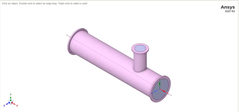
(Mixing T model)
Here we use two type of mesh one is coarse mesh another one is fine mesh; in the coarse mesh we use default mesh size and in the fine mesh use 1mm mesh length with tria element type. We solve the coarse mesh in two methods one is k-epsilon method another one is k-omega method as the given result we use a method for all the simulation.
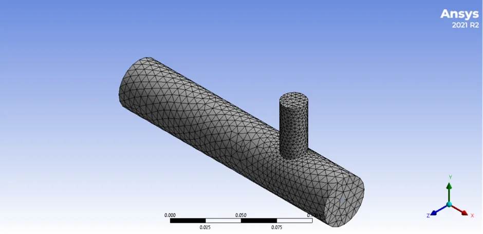
(Coarse mesh of the model)
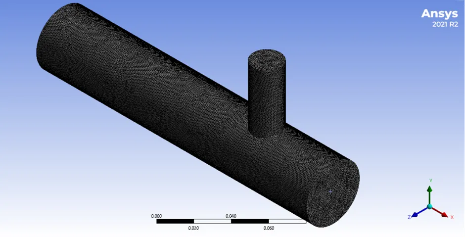
(Fine mesh of the model)

(Quality of the coarse mesh)
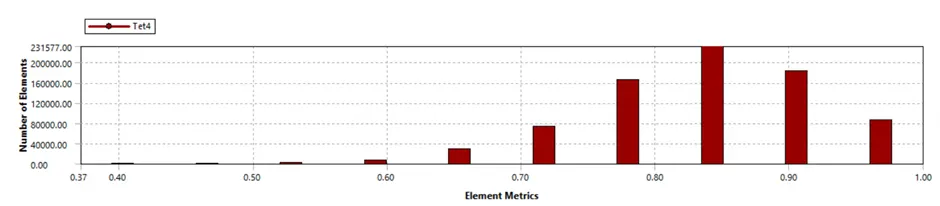
(Quality of the fine mesh)
From the above images, we can see the fine mesh has a better quality of image which is used for future analysis. In the fine mesh, the number of elements is high which will be close to the conserved solution.
Case-1
In our first case, we use 200mm long mixing tee model and the given data are
- Momentum ratio = velocity at cold inlet/velocity at hot inlet
We have momentum ratios are 2, 4 and the hot inlet velocity is 3m/s, so the cold inlet velocity is 6m/s and 12m/s. we have the hot inlet temperature is 36°C and the cold inlet temperature is 19°C. As the given parameter we can open the Ansys fluent and set the all parameters which are required
For the 6m/s velocity at cold inlet, we first consider two simulations with the coarse mesh size elements one is for the k-epsilon realizable model and another one is the k-omega SST model. In the solution, we will considering the standard deviation of the temperature at the outlet and the average weighted temperature at the outlet for both cases.
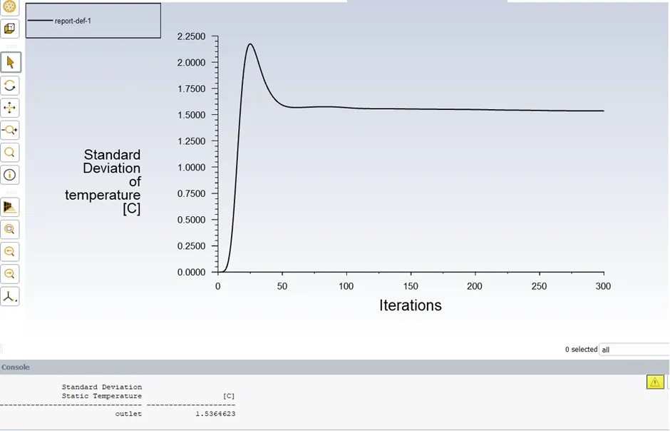
(Standard deviation of temperature for k-epsilon method)
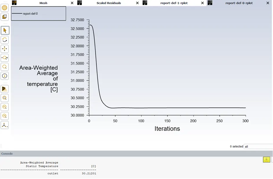
(Area weighted average of temperature for k-epsilon method)
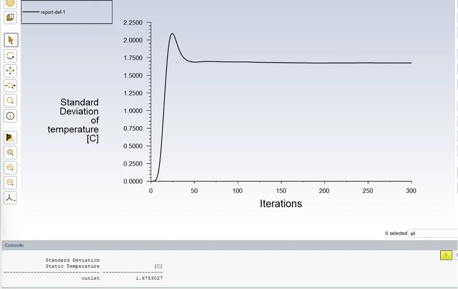
(Standard deviation of temperature for k-omega method)
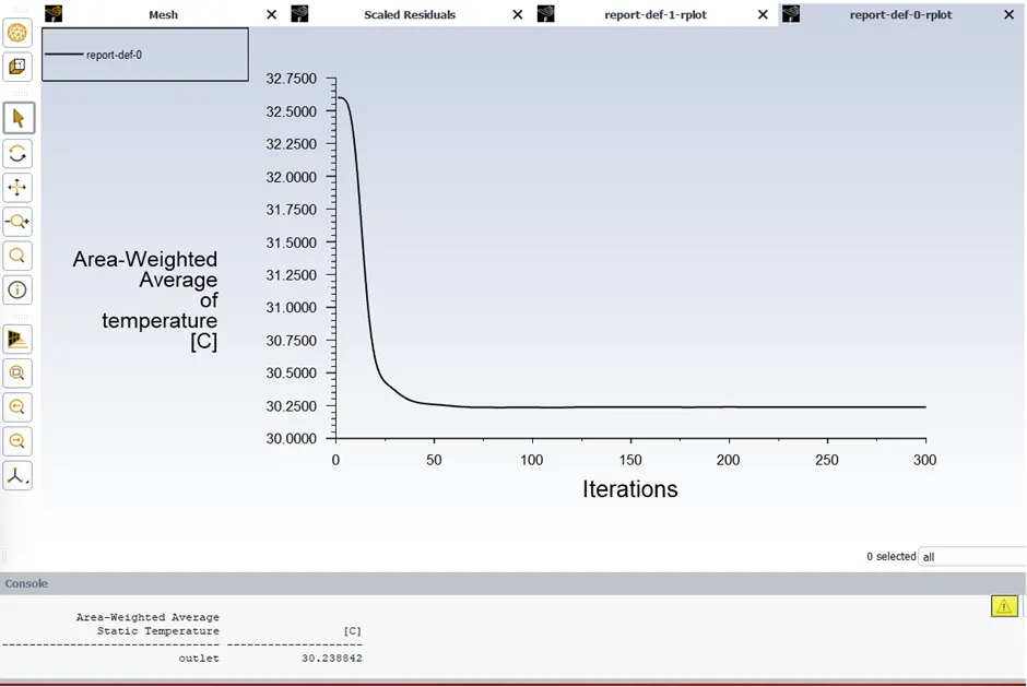
(Area weighted average of temperature for k-epsilon method)
We are getting the result given in the table
|
Methods |
Standard deviation of temperature (°C) |
Area weighted average of temperature (°C) |
|
k-epsilon |
1.5364 |
1.675302 |
|
k-omega |
30.21201 |
30.238842 |
From the table, we can get the result, that the standard deviation temperature is smaller in the k-epsilon methods which will give the result closer to the conserve.
After the coarse mesh simulation, we will go to the fine mesh simulation with the k-epsilon method. Set the hot inlet velocity at 3m/s with 36°C and cold inlet velocity at 6m/s with 19°C temperature air. I have done the hybrid initialization and run the calculation with 200 iterations.
In another simulation, we can take the 12m/s cold inlet velocity with 19°C temperature and hot inlet velocity at 3m/s with 36°C temperature and take the k-epsilon model and take the hybrid initialization and run it with 200 iterations
Case 2
In the 2nd case, we consider the length of the pipe is 300mm with diameter of 40mm and the T joint to be 40mm in length with 20mm diameter. Here we consider only the fine mesh with a mesh length of 1mm. as with the previous momentum ratios 2 and 4 we can define the cold air inlet velocity when the hot inlet velocity is 3m/s.
We can define the cold inlet velocity are 6m/s and 12m/s with the hot air temperature being 36°C and the cold air temperature being 19°C. By these boundary conditions, we can apply the k-epsilon method. We can see the mesh size and quality of the mixing tee.
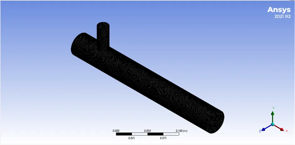
(Mesh with fine elements)
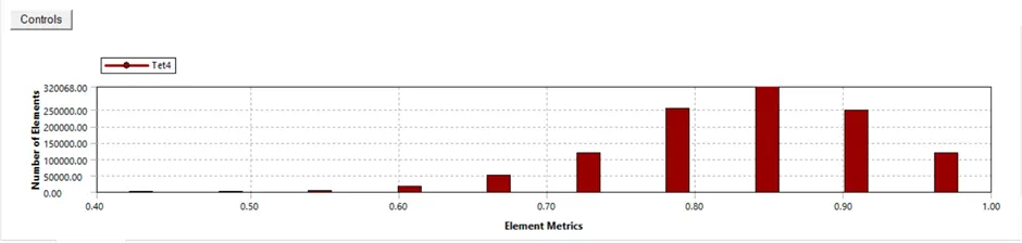
(Mesh quality)
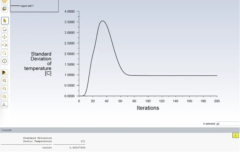
(Standard deviation of temperature for 6m/s cold inlet velocity)
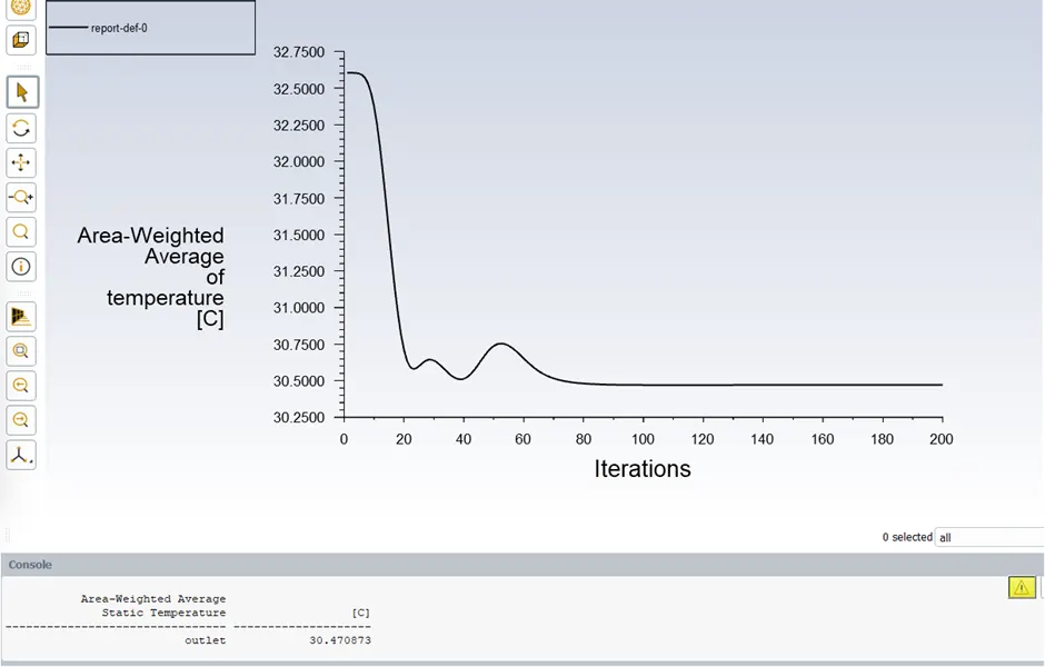
(Area weighted average of temperature for 6m/s cold inlet velocity)
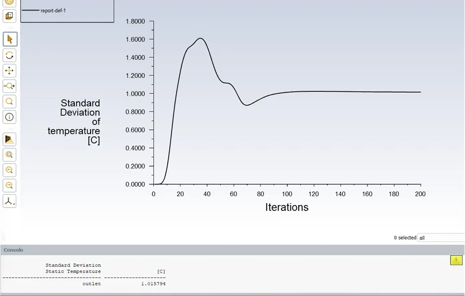
(Standard deviation of temperature for 12m/s cold inlet velocity)
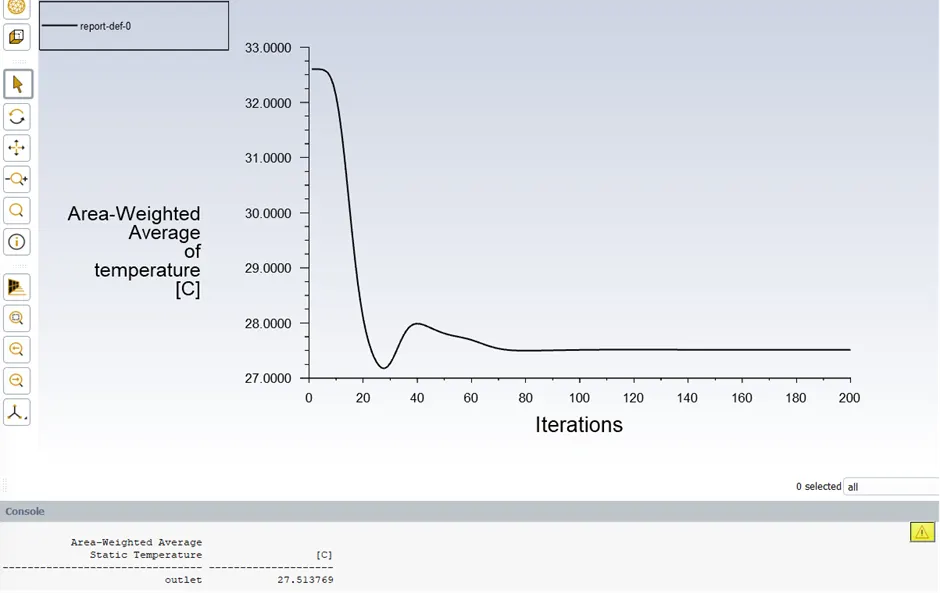
(Area weighted average of temperature for 12m/s cold inlet velocity)
In the above images, we can see the area-weighted average temperature at the outlet and the standard deviation of temperature at the outlet, now we can compare the outlet temperature of the mixing tee.
|
Case |
Cell count |
Average outlet Temperature at 6m/s (°C) |
Average outlet Temperature at 12m/s (°C) |
Number of iterations |
|
Case-1 |
774307 |
30.380962 |
27.633877 |
200 |
|
Case-2 |
1121926 |
30.470873 |
27.513769 |
200 |
Result
After the simulation of the mesh elements, we will get some temperature and velocity which changes with respect to factors like velocity, length of pipe, mesh element sizes, etc. we will discuss both the cases on the fluctuation of temperature and velocity below images present the temperature and velocity profile for the different conditions.
Case-1 result view
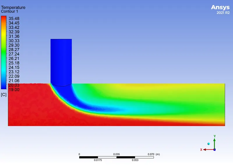
(Temperature counterplot of 6m/s cold inlet velocity)
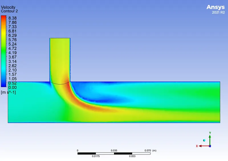
(Velocity counterplot of 6m/s cold inlet velocity)
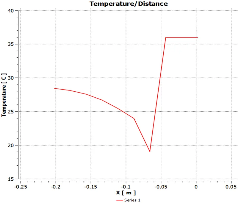
(Temperature v/s Distance graph of 6m/s cold inlet velocity)
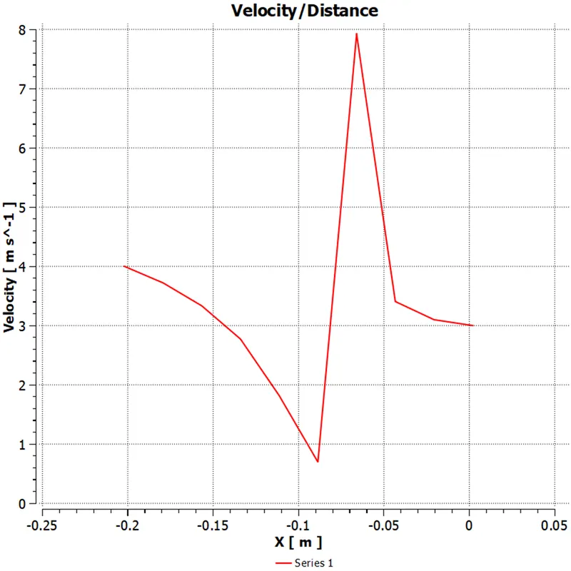
(Velocity v/s Distance graph of 6m/s cold inlet velocity)
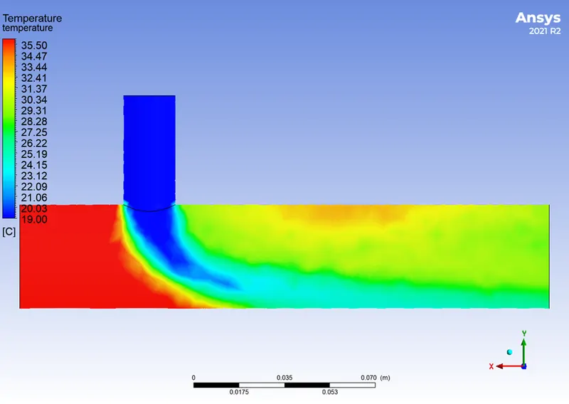
(Temperature counterplot of 12m/s cold inlet velocity)
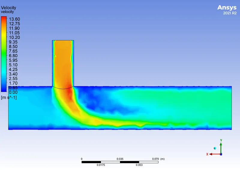
(Velocity counterplot of 12m/s cold inlet velocity)
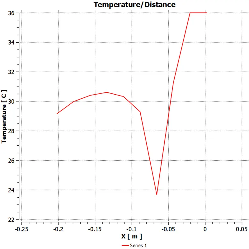
(Temperature v/s Distance graph of 12m/s cold inlet velocity)
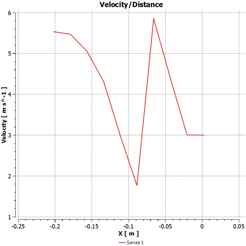
(Velocity v/s Distance graph of 12m/s cold inlet velocity)
Case-2
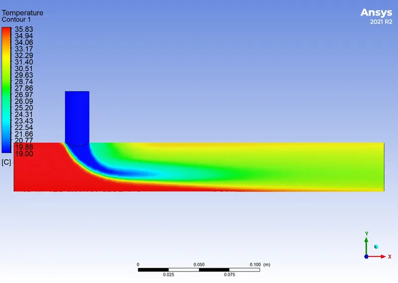
(Temperature counterplot of 6m/s cold inlet velocity)
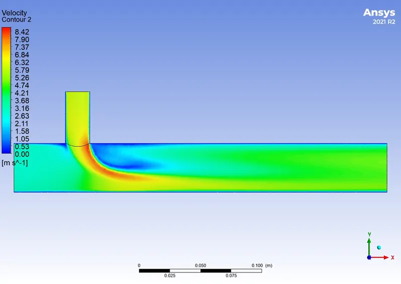
(Velocity counterplot of 6m/s cold inlet velocity)
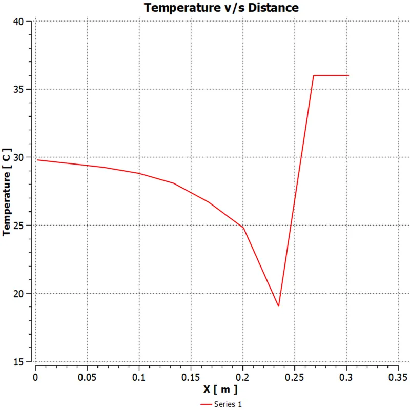
(Temperature v/s Distance graph of 6m/s cold inlet velocity)
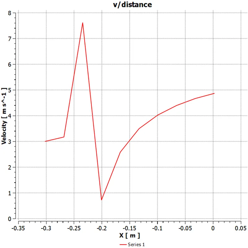
(Velocity v/s Distance graph of 6m/s cold inlet velocity)
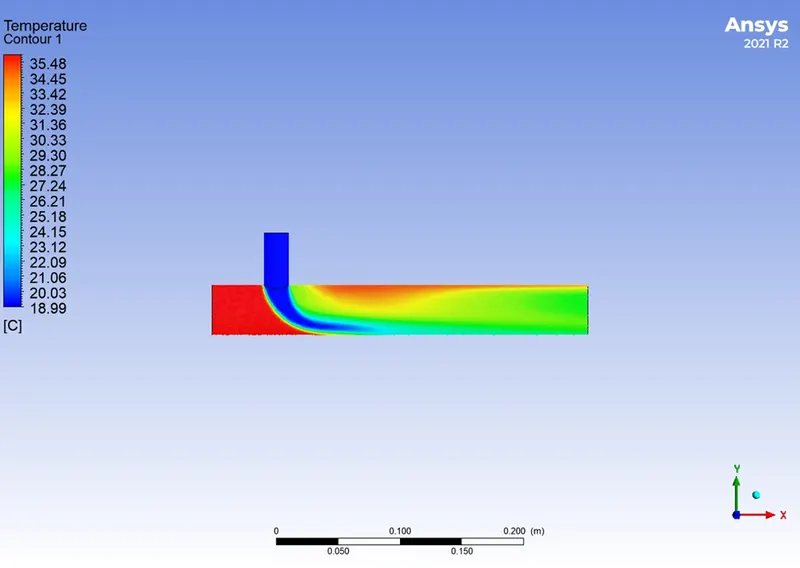
(Temperature counterplot of 12m/s cold inlet velocity)
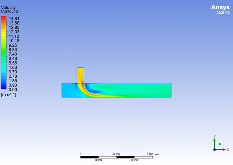
(Velocitycounterplot of 12m/s cold inlet velocity)
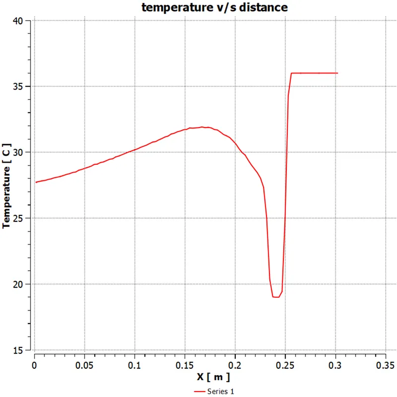
(Temperature v/s Distance graph of 12m/s cold inlet velocity)
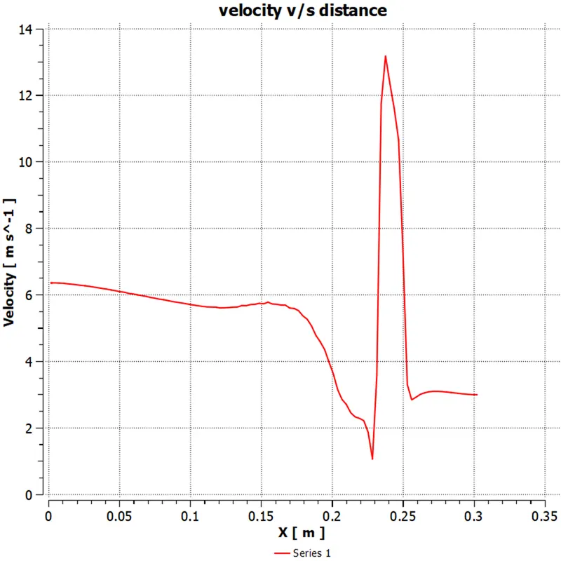
(Velocity v/s Distance graph of 12m/s cold inlet velocity)
Mesh independent study
For the mesh independent study, we consider the two simulations with coarse mesh elements. One mesh element we consider the default mesh size and for another one we consider the 1mm mesh size. We consider the result is counterplot of temperature with mesh gride in the cut plane. Shown in below
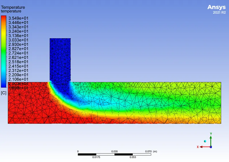
(Temperature counterplot with coarse mesh)
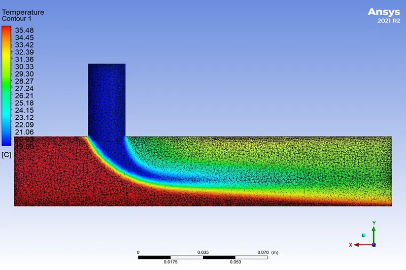
(Temperature counterplot with 1mm mesh size)
We can see the two results in the counterplot here we can easily define the difference, in the default mesh in the mixing junction the temperature variation is not clearly defined but in the fine mesh, we can see the temperature lines are clearly defined. The fluctuation of the temperature after mixing is more in the default mesh model but in the fine mesh, it reduces.
Like mesh, the length of the pipe also gives some effect in this analysis. We can see the below table to check the temperature difference with respect to the length of the pipe
|
length |
Average outlet Temperature at 6m/s (°C) |
Average outlet Temperature at 12m/s (°C) |
|
200 |
30.380962 |
27.633877 |
|
300 |
30.470873 |
27.513769 |
In this table, we can see when the length of the pipe increases the effect of temperature increases because of time for the exchange of heat increases slightly.
Conclusion
In the above analysis, we are able to know how the temperature in the mixing tee is act with respect to the velocity and length of the pipe. Velocity will be different in the different regions which very much fluctuates near the wall which is equal to zero it gradually increases with increasing height; at these places, the heat transfer takes place more. In the mixing line of hot and cold air temperature is fluctuate.
We are using the k-epsilon model to solve the problem which gives a more accurate result in this condition. In the result and discussion, we are able to know much more about how the mesh and other parameters affect the result which is outlet temperature. In the analysis, we can see the hoe the temperature and velocity profile is given. In the turbulence mixing of the model in the T junction, the temperature is defined from the RANS model and it is also compared with the SST model. In our two cases use the RANS model because the SST model gives more different from the RANS model.
Notice: - After the analysis, the size of the file is more, but in the challenge submission time it is not supported because of its large so I am sharing the google drive link please download from the link.
Link: https://drive.google.com/file/d/1z4wRSrWu-h7qFgqIDP9XZvAdbRZ2ShyE/view?usp=drivesdk