Ansys - Mixing Tee
Problem Statement: -
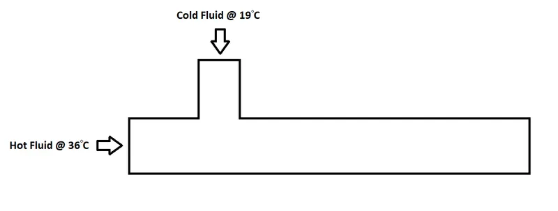
For the Given Mixing Tee Geometries where one is Long and the other is Short. Perform a CFD analysis using Ansys Software when for the given geometry Hot Fluid is entering the Tee along the X direction at `36^@C` and Cold Fluid is entering the Tee along the Y direction at `19^@C`. The Following are the Cases in which analysis needs to be Performed: -
i. Short Tee:-
- The Hot Fluid is entering along X direction at 3 m/sec.
- Perform analysis for two cases when Momentum Ration is 2 and 4
ii. Long Tee:-
- The Hot Fluid is entering along X direction at 3 m/sec.
- Perform analysis for two cases when Momentum Ration is 2 and 4
Note: Momentum Ratio `= (V_(cold))/(V_(hot))`
Expected Results: -
- Develop an Analytical Solution for the same to have a basis for Comparision.
- Compare the Results to provide conclusions about different Mixing Lengths and Mixing Velocities.
Solution: -
1. AIM: -
A. For the given Long and Short Mixing Tee perform CFD Analysis using Ansys and Explain the Results.
B. Compare the results of the Simulation with the Analytical Solution.
2. Given and Assumed: -
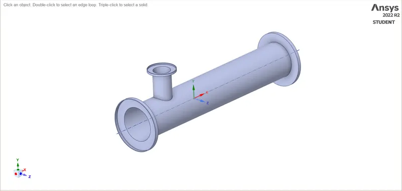
A. Short Tee: -
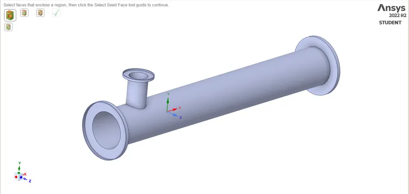
B. Long Tee: -
C. Fluid Inlet Conditions: -
D. For the Following Parameters the Following Symbols are used: -
i. The Area of Pipe `->` `A`
ii. The diameter of Pipe `->` `d`
iii. The density of The Fluid `->` `rho`
iv. The velocity of The Fluid `->` `V`
v. The Total Energy of The Fluid `->` `E`
vi. The Specific Internal Energy of The Fluid `->` `u`
vii. The Specific Enthalpy of The Fluid `->` `h`
viii. The Temperature of The Fluid `->` `T`
ix. The Specific Heat at Constant Pressure of The Fluid `->` `c_p`
x. The Specific Volume of The Fluid `->` `v`
xi. The Ratio of Specific Heat of The Fluid `->` `gamma`
xii. The Momentum Ratio `->` `(M.R.) = V_(cold)/V_(hot)`
E. Denotation and Values that are given for different Locations: -
i. Denotation of Parameters in Pipe 1(The Pipe where Hot Fluid is Entering) `-> phi_1`
ii. Denotation of Parameters in Pipe 2(The Pipe where Cold Fluid is Entering) `-> phi_2`
iii. The Velocity of Hot Fluid inlet`(V_(hot)) =` 3 m/sec
iv. Momentum Ratio For each Short and Long Mixing Tee = 2 and 4
F. Materials of The Process: -
i. The Working Fluid `->` Air
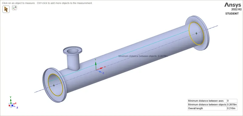
3. Measuring the Dimensions of Mixing Tees: -
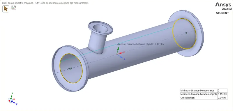
A. Short Tee:-
i. Diameter of Hot Fluid Entry `->` 34mm
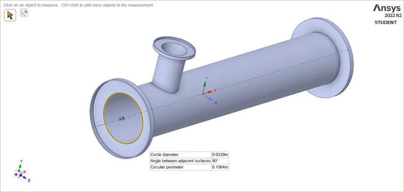
ii. Diameter of Hot Fluid Entry `->` 17mm
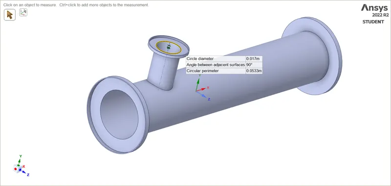
iii. Length of Pipe 1 of Hot Fluid Entry `->` 192mm
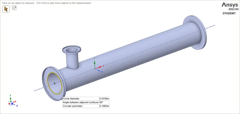
B. Long Tee: -
i. Diameter of Hot Fluid Entry `->` 34mm
ii. Diameter of Hot Fluid Entry `->` 17mm
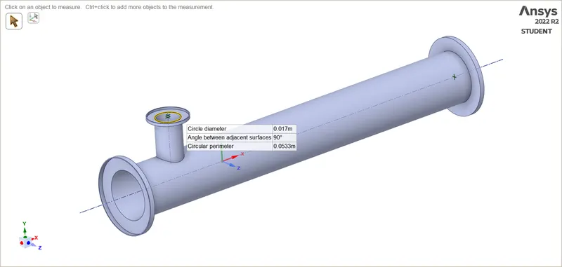
iii. Length of Pipe 1 of Hot Fluid Entry `->` 268mm
4. Analytical Solution: -
The Analytical Solution can be calculated by taking the Following Assumptions:-
i. The Process is Quasi-Static
ii. The Fluid is an ideal Fluid
iii. There are no frictional Losses
iv. The Process is Steady State
By taking the above-given Assumptions the given Situation will have the following Characteristics: -
i. The Process will be reversible and Homogeneous.
ii. The Values of Specific heat of the Fluid will be Constant.
Taking the Given Mixing Tee as a Control Volume with Perfectly Insulated Boundary(Or Adiabatic Boundary) and No Work Transfer across the Boundary. Performing mass and Energy Conservation for the System: -
A. Mass Conservation: -
As it is a Steady State System, The Total Mass inlet in the Control Volume will be Equal to the Total Mass leaving the System
`=> dot(m)_(cold) + dot(m)_(hot) = dot(m)_("outlet")`
`=> rho_(cold)A_2V_(cold) + rho_(hot)A_1V_(hot) = rho_("outlet")A_1V_("outlet")`
`=> rho_(cold)(pi/4d_2^2)V_(cold) + rho_(hot)(pi/4d_1^2)V_(hot) = rho_("outlet")(pi/4d_1^2)V_("outlet")`
`=> rho_(cold)(d_2^2)V_(cold) + rho_(hot)(d_1^2)V_(hot) = rho_("outlet")(d_1^2)V_("outlet")`
Now,
Dividing Both Sides with `rho_("outlet")(d_1^2)`
`=> (rho_(cold)/rho_("outlet"))(d_2^2/(d_1^2))V_(cold) + (rho_(hot)/rho_("outlet"))V_(hot) = V_("outlet") " "-> bb((eq. 1))`
Now,
As the Process is Reversible and Adiabatic
So,
`v_("outlet")/(v_(cold)) = (T_(cold)/T_("outlet"))^(1/(gamma-1))`
And,
As `rho = 1/v`
`=> rho_(cold)/(rho_("outlet")) = (T_(cold)/T_("outlet"))^(1/(gamma-1)) " "-> bb((eq. 2))`
Similarly,
`=> rho_(hot)/(rho_("outlet")) = (T_(hot)/T_("outlet"))^(1/(gamma-1)) " "-> bb((eq. 3))`
Now,
Putting the Values of `(eq. 2)` and `(eq. 3)` in `(eq. 1)`
`=> (T_(cold)/T_("outlet"))^(1/(gamma-1))(d_2^2/(d_1^2))V_(cold) + (T_(hot)/T_("outlet"))^(1/(gamma-1))V_(hot) = V_("outlet") " "-> bb((eq. 4))`
B. Energy Conservation: -
As it is a Steady State System, The Total Energy Entering the Control Volume is Equal to the Total Energy Exiting the System
`((dU)/(dt))_("Control Volume") = dot(E)_("inlet") - dot(E)_("Outlet")`
Now,
As The System is in Steady State `(=> ((dU)/(dt))_("Control Volume") = 0)`
`=> dot(E)_("inlet") - dot(E)_("Outlet") = 0`
`=> dot(E)_("inlet") = dot(E)_("Outlet")`
`=> dot(m)_("inlet")h_("inlet") = dot(m)_("Outlet")h_("Outlet")`
`=> dot(m)_(cold)h_(cold) + dot(m)_(hot)h_(hot) = dot(m)_("Outlet")h_("Outlet")`
`=> (rho_(cold)A_2V_(cold))(c_pT_(cold)) + (rho_(hot)A_1V_(hot))(c_pT_(hot)) = (rho_("outlet")A_1V_("outlet"))(c_pT_("Outlet"))`
`=> (rho_(cold)A_2V_(cold))(T_(cold)) + (rho_(hot)A_1V_(hot))(T_(hot)) = (rho_("outlet")A_1V_("outlet"))(T_("Outlet"))`
`=> (rho_(cold)(pi/4d_2^2)V_(cold))(T_(cold)) + (rho_(hot)(pi/4d_1^2)V_(hot))(T_(hot)) = (rho_("outlet")(pi/4d_1^2)V_("outlet"))(T_("Outlet"))`
`=> (rho_(cold)(d_2^2)V_(cold))(T_(cold)) + (rho_(hot)(d_1^2)V_(hot))(T_(hot)) = (rho_("outlet")(d_1^2)V_("outlet"))(T_("Outlet"))`
Now,
Dividing Both Sides with `rho_("outlet")(d_1^2)`
`=> (rho_(cold)/rho_("outlet"))(d_2^2/d_1^2)V_(cold)(T_(cold)) + (rho_(hot)/rho_("outlet"))V_(hot)(T_(hot)) = (V_("outlet"))(T_("Outlet")) " "bb((eq. 5))`
Now,
Putting the Value of `(eq. 2)` `[rho_(cold)/(rho_("outlet")) = (T_(cold)/T_("outlet"))^(1/(gamma-1))]` and `(eq. 3)` `[rho_(hot)/(rho_("outlet")) = (T_(hot)/T_("outlet"))^(1/(gamma-1))]` in `(eq. 5)`
`=> (T_(cold)/T_("outlet"))^(1/(gamma-1))(d_2^2/d_1^2)V_(cold)(T_(cold)) + (T_(hot)/T_("outlet"))^(1/(gamma-1))V_(hot)(T_(hot)) = (V_("outlet"))(T_("Outlet"))`
`=> (1/T_("outlet"))^(1/(gamma-1))[(T_(cold))^(gamma/(gamma-1))(d_2^2/d_1^2)V_(cold) + (T_(hot))^(gamma/(gamma-1))V_(hot)] = (V_("outlet"))(T_("Outlet")) " "bb((eq. 6))`
C. Calculating Velocity and Temperature at the Outlet: -
Dividing `(eq. 4)` from `(eq. 6)`
`((1/T_("outlet"))^(1/(gamma-1))[(T_(cold))^(gamma/(gamma-1))(d_2^2/d_1^2)V_(cold) + (T_(hot))^(gamma/(gamma-1))V_(hot)])/((1/T_("outlet"))^(1/(gamma-1))[(T_(cold))^(1/(gamma-1))(d_2^2/d_1^2)V_(cold) + (T_(hot))^(1/(gamma-1))V_(hot)]) = T_("outlet")`
`=> ((T_(cold))^(gamma/(gamma-1))(d_2^2/d_1^2)V_(cold) + (T_(hot))^(gamma/(gamma-1))V_(hot))/((T_(cold))^(1/(gamma-1))(d_2^2/d_1^2)V_(cold) + (T_(hot))^(1/(gamma-1))V_(hot)) = T_("outlet")`
Now,
Dividing Numerator and Denemonetor on L.H.S. with `V_(hot)`
`=> ((T_(cold))^(gamma/(gamma-1))(d_2^2/d_1^2)(V_(cold)/V_(hot)) + (T_(hot))^(gamma/(gamma-1)))/((T_(cold))^(1/(gamma-1))(d_2^2/d_1^2)(V_(cold)/V_(hot)) + (T_(hot))^(1/(gamma-1))) = T_("outlet")`
Now,
As Given that `(V_(cold)/V_(hot)) = (M.R.)`
`=> T_("outlet") = ((T_(cold))^(gamma/(gamma-1))(d_2^2/d_1^2)(M.R.) + (T_(hot))^(gamma/(gamma-1)))/((T_(cold))^(1/(gamma-1))(d_2^2/d_1^2)(M.R.) + (T_(hot))^(1/(gamma-1))) " "bb((eq. 7))`
Now,
As `T_(cold) = 292.15K`, `T_(hot) = 309.15K`, `d_1 = 34 m` and `d_2 = 17 m`
Case 1: Momentum Ratio = 2: -
From `(eq. 7)`
`T_("(Outlet @ MR = 2)") = 304K` or `30.85^@C`
From `(eq. 4)` and `T_("(Outlet @ MR = 2)")`
`V_("(Outlet @ MR = 2)") = 4.49` m/sec
Case 2: Momentum Ratio = 4: -
From `(eq. 7)`
`T_("(Outlet @ MR = 4)") = 301.25K` or `28.10^@C`
From `(eq. 4)` and `T_("(Outlet @ MR = 4)")`
`V_("(Outlet @ MR = 4)") = 5.98` m/sec
| Analytical Solution |
| Momentum Ratio | Momentum Ratio = 2 | Momentum Ratio = 4 |
| Velocity @ Outlet | 4.49 m/sec | 5.98 m/sec |
| Temperature @ Outlet | `30.85^@C` | `28.10^@C` |
5. Steps to Perform Analysis For Any Mixing Tee: -
A. Setting up The Workbench:-
i. Steps to Create a Project: -
Ansys Workbench`->`ToolBox`->`Analysis Systems`->``ubrace("Fluid Flow (Fluent)")_["Selecting"->"Holding" ->"Dragging and Dropping to Project Schematic"]`
B. Opening SpaceClaim Geometry and Extracting Volume: -
i. Steps to Open SpaceClaim: -
Ansys Workbench `->` Project Schematic `->` Project `->` Geometry `->` Right-Click `->` Select SpaceClaim Geometry
ii. Steps to Load the Geometry: -
SpaceClaim `->` File `->` Open
iii. Steps to Extract Volume: -
SpaceClaim `->` Prepare `->` Volume Extract `->` Select Edges `->` Enter
iv. Steps to Suppress for Physics of Solid Surface: -
SpaceClaim `->` Structure Window `->` Select the Component `->` Right-Click `->` Suppress for Physics
C. Opening Mechanical(Meshing) and Meshing the Geometry: -
i. Steps to Open Meshing: -
Ansys Workbench `->` Project Schematic `->` Project `->` Mesh `->` Right-Click `->` Edit
ii. Steps to Name the Boundary: -
Mechanical(Meshing) `->` Model Working Window `->` Select the Boundary `->` Click N `->` Give the desired Name `->` Enter
iii. Steps to Create Mesh: -
Mechanical(Meshing) `->` Outline Window `->` Select Mesh `->` Details of Mesh Window `->` Defaults `->` Element Size `->` Give Desired Element Size `->` Outline Window `->` Mesh `->` Right-Click `->` Generate Mesh
D. Opening Ansys Fluent and Performing Analysis: -
i. Steps to Open Ansys Fluent: -
Ansys Workbench `->` Project Schematic `->` Project `->` Setup `->` Right-Click `->` Edit
ii. Steps to Check Mesh: -
Fluent `->` Outline View Window `->` Setup `->` General `->` Mesh `->` Check
iii. Steps to Set up the Physics: -
a. Fluent `->` Physics `->` Models `->` Tick Energy Box
b. Fluent `->` Physics `->` Models `->` Viscous `->` Select Desired Viscous Model `->` Enter
iv. Steps to Set up Material, Cell Zone Condition, and Boundary Condition: -
a. Fluent `->` Physics `->` Materials `->` Create/Edit... `->` Select/Create the desired Fluid `->` Enter
b. Fluent `->` Physics `->` Zone `->` Cell Zone `->` Select the desired Component `->` Edit `->` Make the desired Change `->` Enter
c. Fluent `->` Physics `->` Zone `->` Boundaries `->` Select the desired Component `->` Select the Desired Type for that Component `->` Edit `->` Add the Values for the Component `->` Apply & Close
v. Steps to Set up Reports: -
Fluent `->` Solution `->` Reports `->` Definition `->` New `->` Select the Desired Report `->` Rename the Report `->` Change the Field Variable to Desired Variable `->` Select the desired Surface `->` Ok
vi. Steps to Run Analysis: -
a. Fluent `->` Solution `->` Initialization `->` Initialize
b. Fluent `->` Solution `->` Run Calculations `->` No. of Iterations `->` Set to desired Iterations
b. Fluent `->` Solution `->` Run Calculations `->` Calculate
E. Opening Ansys Fluent and Creating Desired Graphical Reports: -
i. Steps to Open Ansys Fluent: -
Ansys Workbench `->` Project Schematic `->` Project `->` Solution `->` Right-Click `->` Edit
ii. Steps to Add a XY Plane: -
Fluent `->` Results `->` Surface `->` Create `->` Plane `->` Rename `->` Select Method to XY Plane `->` Create
iii. Steps to Create Contours: -
Fluent `->` Results `->` Graphics `->` Contours `->` New `->` Rename `->` Select Variable for Contour of `->` Select Surface `->` Save/Display
iv. Steps to Create Vectors: -
Fluent `->` Results `->` Graphics `->` Vectors `->` New `->` Rename `->` Select Variable for Vectors of `->` Select Surface `->` Save/Display
v. Steps to Create Pathlines: -
Fluent `->` Results `->` Graphics `->` Pathlines `->` New `->` Rename `->` Select Style and give its parameters `->` Select Color of `->` Select Surface `->` Save/Display
vi. Steps to Create Report Outline: -
Fluent `->` Outline View `->` Simulation Reports `->` Report Outline `->` Rename Report Name `->` Select Desired Report Components from Report Section `->` Generate
6. Outputs Generated after Each Step before Analysis for Short Tee: -
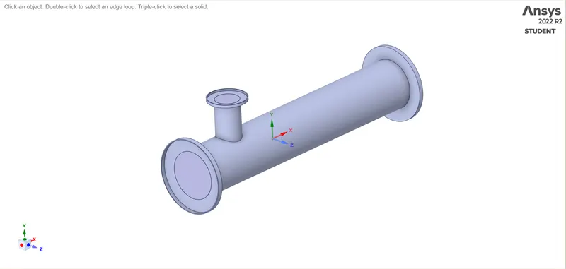
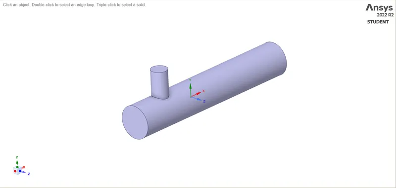
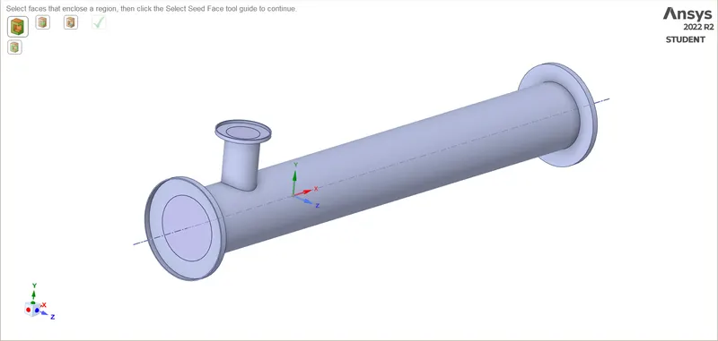
A. Geometry: -
i. After Loading Geometry: -
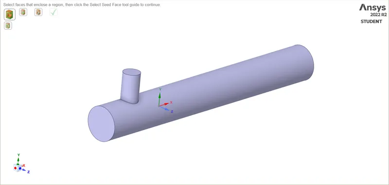
ii. After Extracting Volume: -
B. Meshing: -
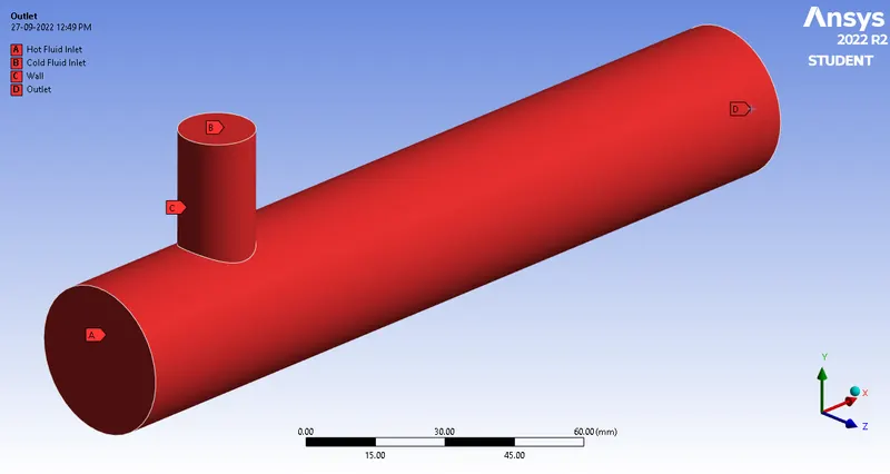
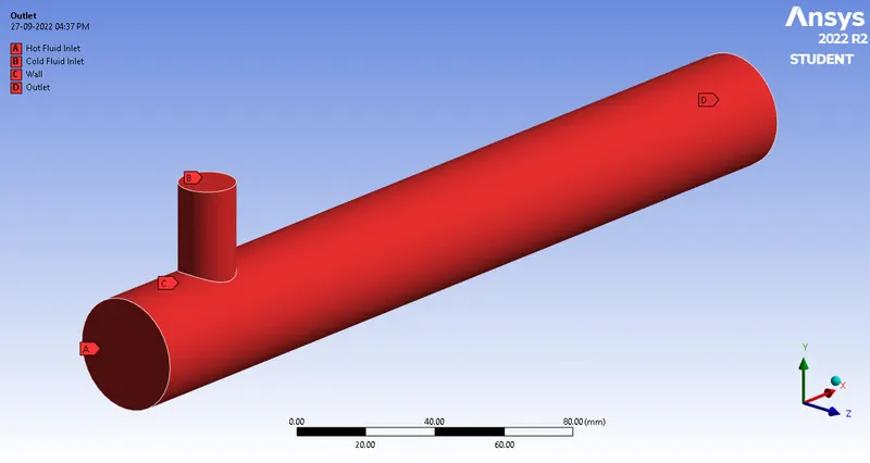
i. After Naming the Boundaries: -
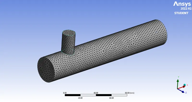
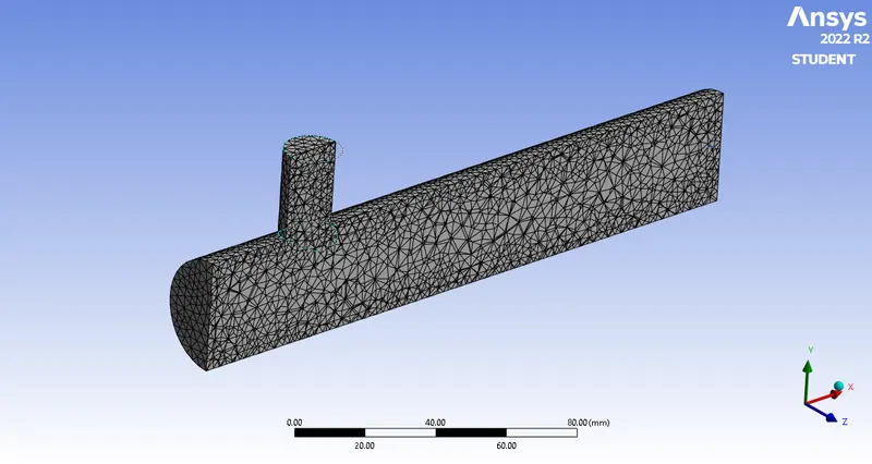
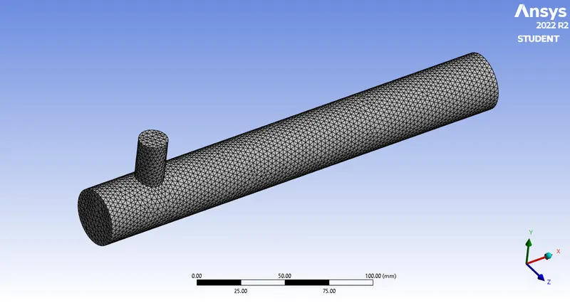
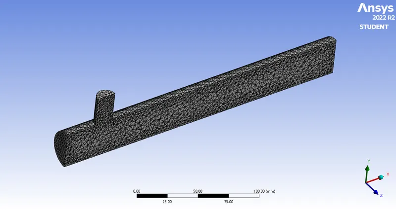
ii. After Meshing: -
C. Setup: -
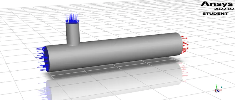
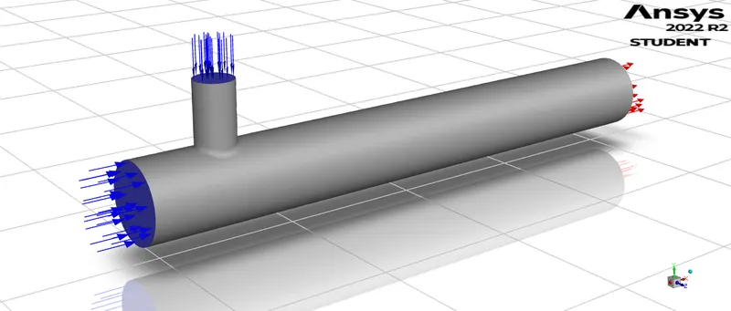
i. After Loading in Fluent: -
7. Outputs/Results Generated after Analysis in Short Mixing Tee: -
A. Case 1: For Momentum Ratio = 2: -
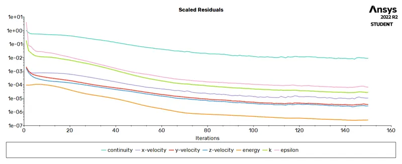
i. Calculations Done while Iterations: -
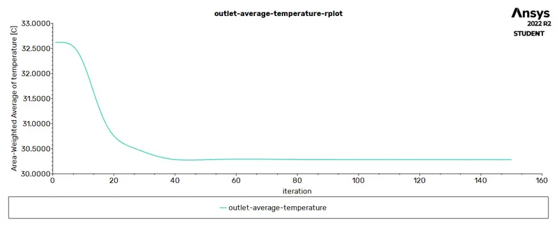
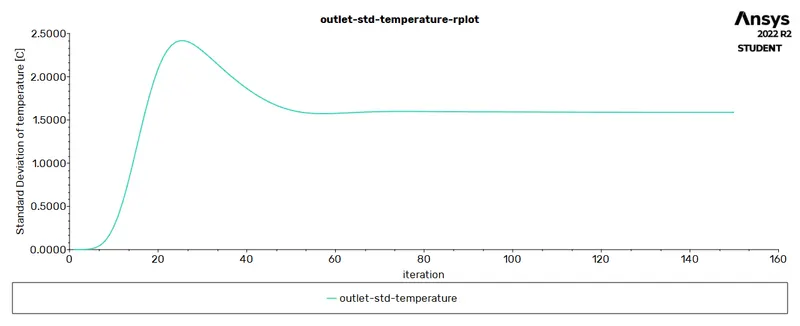
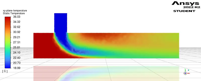
ii. The Temperature and Velocity Contours: -
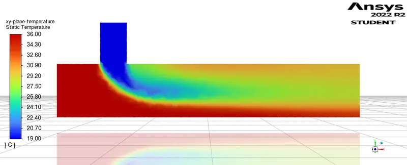
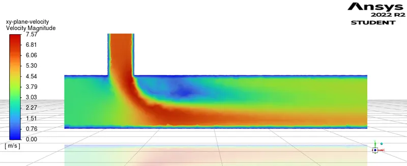
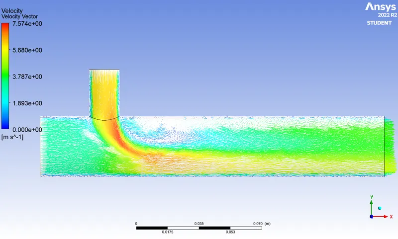
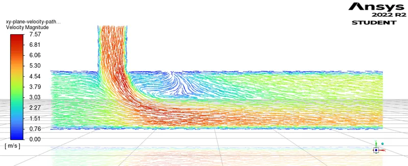
iii. The Velocity Vectors and Pathlines: -
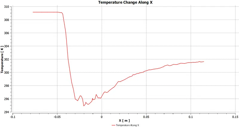
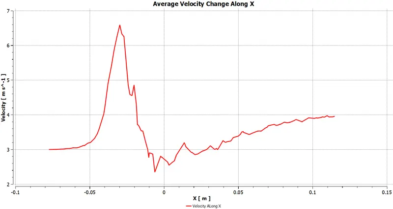
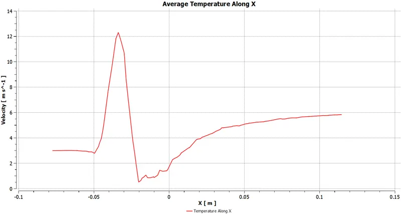
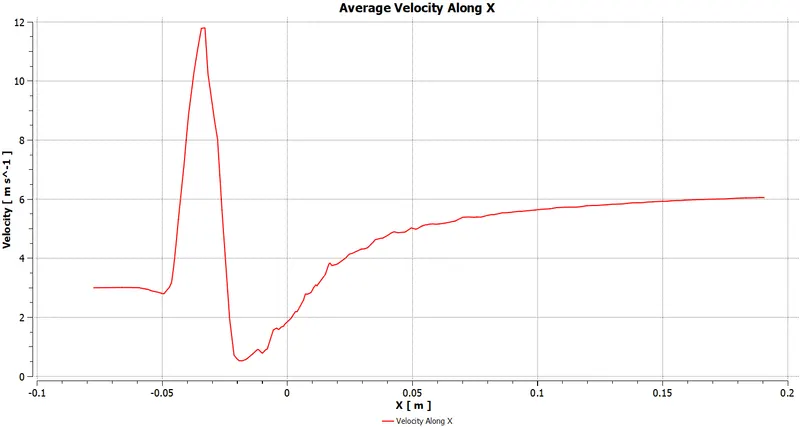
iv. The Average Temperature and Average Velocity Plot along X dir: -
B. Case 2: For Momentum Ratio = 4: -
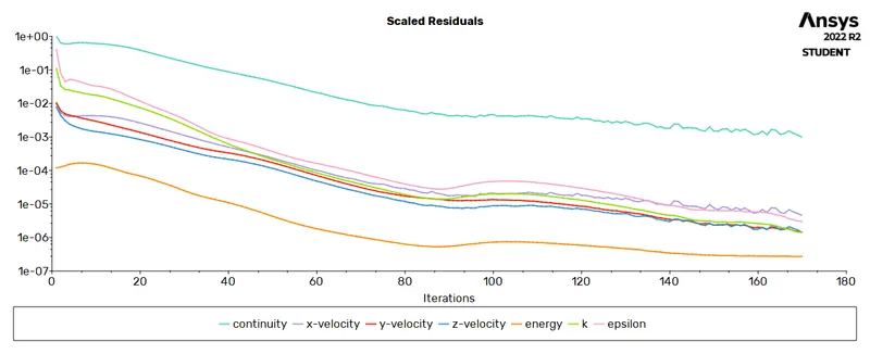
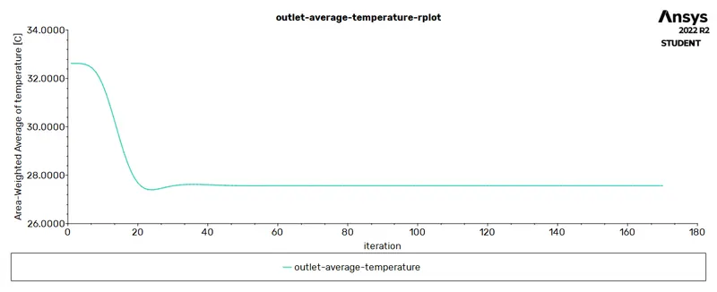
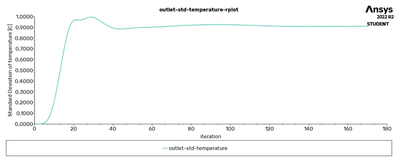
i. Calculations Done while Iterations: -
ii. The Temperature and Velocity Contours: -
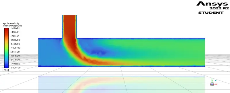
iii. The Velocity Vectors and Pathlines: -
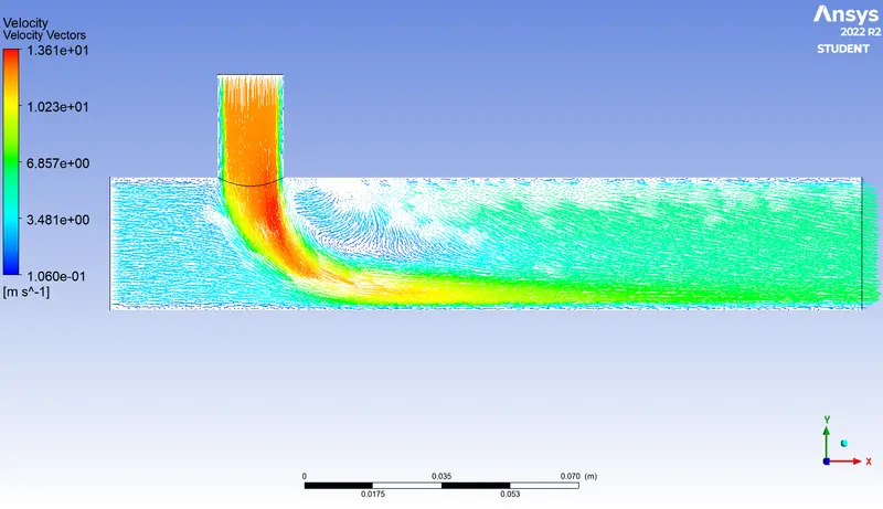
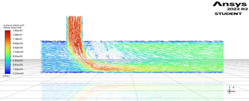
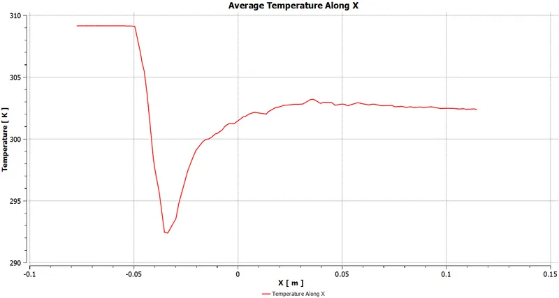
iv. The Average Temperature and Average Velocity Plot along X dir: -
8. Outputs Generated after Each Step before Analysis for Short Tee: -
A. Geometry: -
i. After Loading Geometry: -
ii. After Extracting Volume: -
B. Meshing: -
i. After Naming the Boundaries: -
ii. After Meshing: -
C. Setup: -
i. After Loading in Fluent: -
9. Outputs/Results Generated after Analysis in Long Mixing Tee: -
A. Case 1: For Momentum Ratio = 2: -
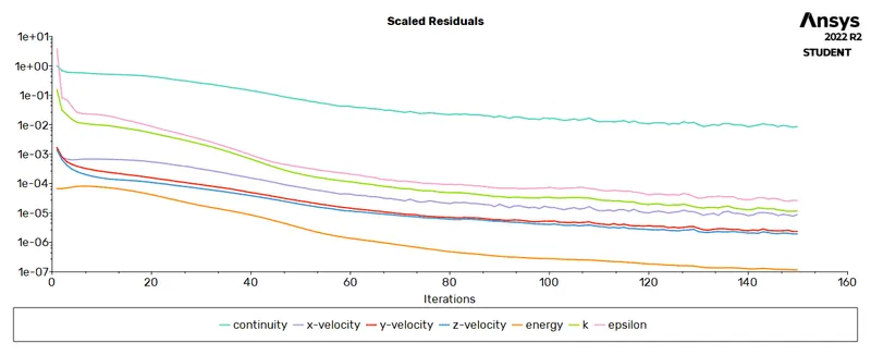
i. Calculations Done while Iterations: -
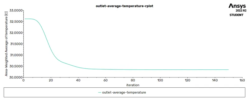
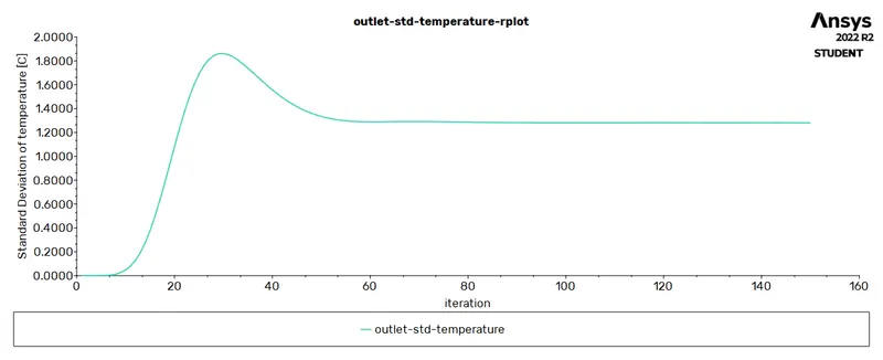
ii. The Temperature and Velocity Contours: -
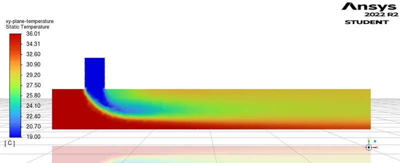
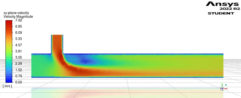
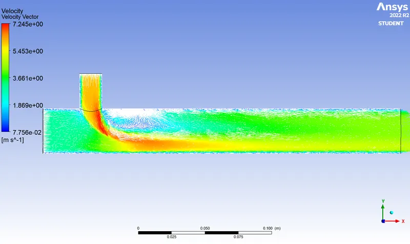
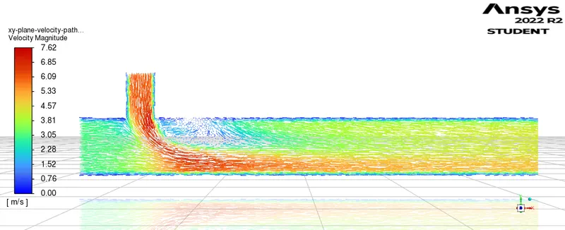
iii. The Velocity Vectors and Pathlines: -
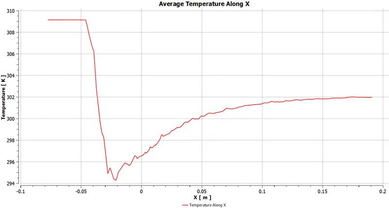
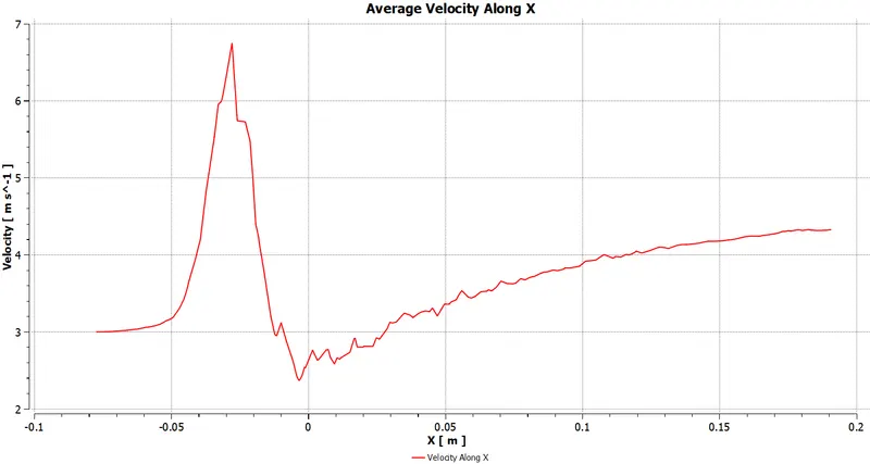
iv. The Average Temperature and Average Velocity Plot along X dir: -
B. Case 2: For Momentum Ratio = 4: -
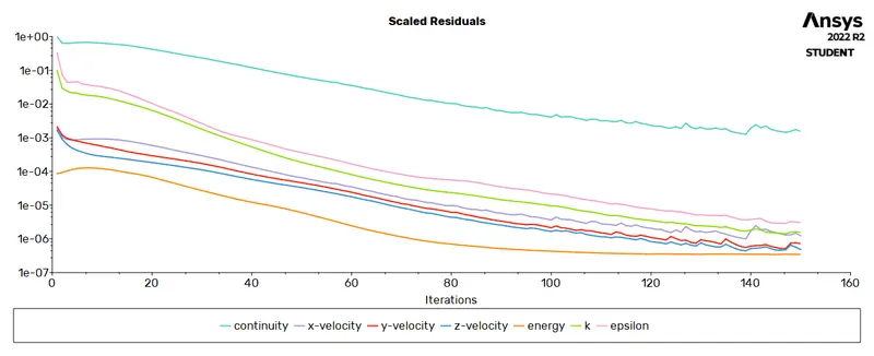
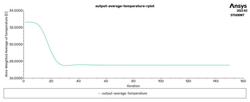
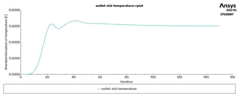
i. Calculations Done while Iterations: -
ii. The Temperature and Velocity Contours: -
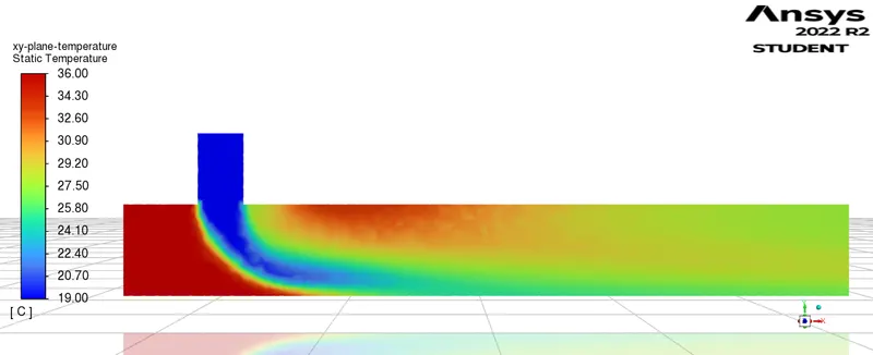
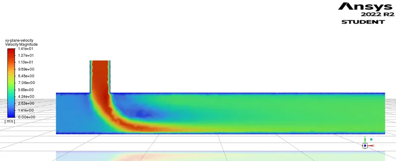
iii. The Velocity Vectors and Pathlines: -
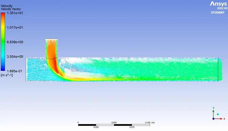
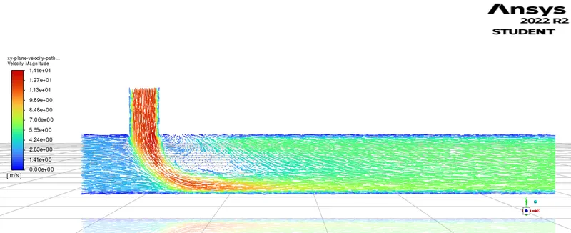
iv. The Average Temperature and Average Velocity Plot along X dir: -
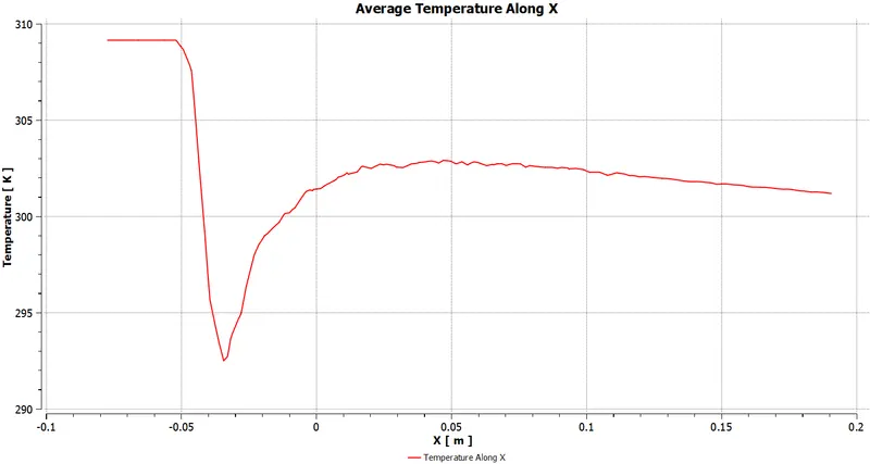
10. Conclusions: -
A. Effect of Length on the Mixing: -
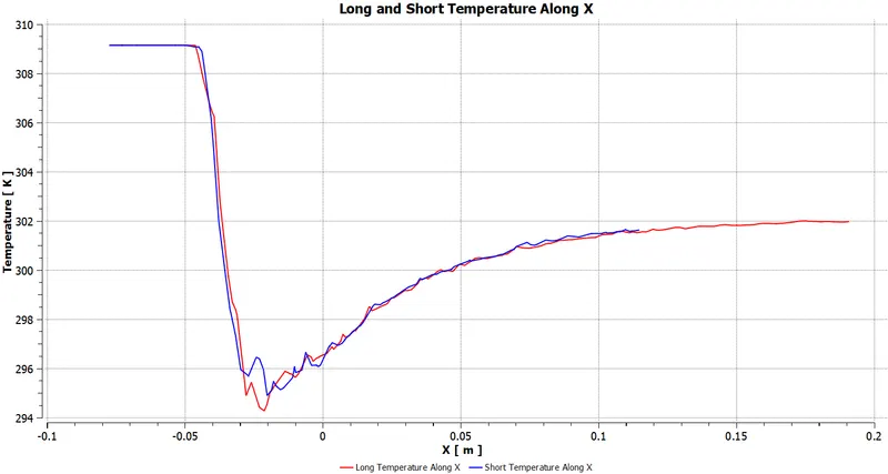
The above comparison between Short and Long Mixing Tee Shows that the Temperature attained at the Outlet of each mixing Tee is still developing towards an equilibrium Temperature and with more length, the mixing at the Outlet will become more homogeneous.
| Mixing Efficiency `bb(alpha)` Length |
B. Effect of Momentum Ratio on the Mixing: -
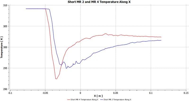
The above comparison between Momentum Ratio = 2 and 4 respectively for Short Mixing Tee Shows that the Temperature attained at the Outlet of each mixing Tee is still developing towards an equilibrium Temperature and with more Momentum Ratio, the mixing at the Outlet will become more homogeneous.
| Mixing Efficiency `bb(alpha)` Momentum Ratio between Both the Fluids |