Week 1- Mixing Tee

AIM:

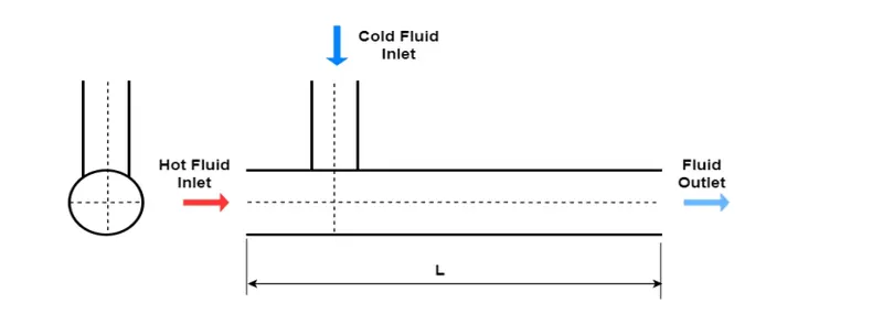
For the given two versions(short and long) of the mixing tree model we are performing the steady-state simulations using the (K-epsilon/K-omega SST) model to compare the mixing effectiveness when the hot inlet temperature is 36⁰C & the Cold inlet is 19⁰C. Determine the temperature and velocity distribution along the mixing tree model.

OBJECTIVES:

In the mixing tree model hot and cold fluid (air) is entered which is a steady-state simulation using the (K-epsilon/K-omega SST) model and compare the mixing effectiveness when the hot inlet temperature is 36°C & the Cold inlet is at 19°C. Our primary focus is the best model suitable for mixing effectiveness to determine the temperature and velocity at the outlet of the cylinder and obtain Velocity and temperature contour plots, with graph variation of Velocity and temperature along the length of the cylinder for both short and long mixing tree models.

THEORY AND CALCULATIONS:

Thermal mixing(T-joints) phenomena are important in many applications such as refrigeration, nuclear power plant, air conditioning, etc. For example, let us consider air conditioning in order to get the desired temperature for the room we cannot use cold air completely hence we are taking normal air from the atmosphere and mixing it with the cold air to get the desired temperature for the room. We are performing the same phenomena as air conditioning but instead Here we are using Hot and cold fluids(different temperatures) for thermal mixing also we are using the turbulence modeling technique (K-epsilon/K-omega) to get standard converged results for temperature and velocity at the end of the pipe. Once the simulations are performed we check for standard deviation to check the mixing effectiveness. Finally, I check for the temperature and velocity obtained from the simulation and compare these results with the theoretical temperature and velocity calculated results.

MASS BALANCE EQUATION

The mass flow rate of working fluid(AIR)= `rho*A*V ((Kg)/s)`

The mass flow rate at outlet[total mass flow]= mass flow rate of hot fluid+mass flow rate of cold fluid.

`rhom*Am*Vm= rhoh*Ah*Vh+ rhoc*Ac*Vc`

Since density is the same it cancels out.

hence

`Dm^2*Vm= Dh^2*Vh+Dc^2*Vc`

`Vm=(Dh^2*Vh+Dc^2*Vc)/(Dm^2)`

ENERGY BALANCE EQUATION

Heat flow in the cylinder(H)=Cp*T

`Hm*Mm= Hh*mh+ Hc*mc`

Cp is common and cancels out on both ends.

`Tm*Mm= Th*mh+Tc*mc`

`Tm= (Th*mh+Tc*mc)/(Mm)`

GEOMETRY PARAMETERS

Diameter of Hot fluid inlet = 33.87m.

Diameter of cold fluid inlet = 16.96m.

Length of the mixing tree = 192.37m.

Hot inlet velocity = 3m/s.

Momentum ratio = velocity at cold inlet / velocity at hot inlet.

velocity at cold inlet = momentum ratio * velocity at hot inlet.

For momentum ratio=2,

the velocity at cold inlet= 2*3= 6m/s.

For momentum ratio=4,

the velocity at cold inlet= 4*3= 12m/s.

For momentum ratio=2

`Vm=(Dh^2*Vh+Dc^2*Vc)/(Dm^2)`

By substituting the above parameters into the equations we find the outlet velocity

`Vm=((33.87)^2*3+(16.96)^2*6)/((33.87)^2)`

Vm= 4.5m/s

`Tm= (Th*mh+Tc*mc)/(Mm)`

`mh=rho(air)*A(hot)*Vh` `mc=rho(air)*A(cold)*Vc`

`mh=1.2*(pi/4)*d^2*3` `mc=1.2*(pi/4)*d^2*6`

`mh=1.2*(pi/4)*(33.87)^2*3` `mc=1.2*(pi/4)*(16.96)^2*6`

mh= 3232.08 (Kg/s) mc= 1626.5 (Kg/s)

Mm= mh+mc

Mm= 3232.08+1626.5= 4858.65 (Kg/s)

The temperature of hot fluid is 36C and the temperature of cold fluid is 19C

`Tm= (Th*mh+Tc*mc)/(Mm)`

`Tm= (36*3232.08+19*1626.5)/(4858.65)`

Tm= 30.30C.

For momentum ratio=4

`Vm=(Dh^2*Vh+Dc^2*Vc)/(Dm^2)`

By substituting the above parameters into the equations we find the outlet velocity

`Vm=((33.87)^2*3+(16.96)^2*12)/((33.87)^2)`

Vm= 6.008m/s

`Tm= (Th*mh+Tc*mc)/(Mm)`

`mh=rho(air)*A(hot)*Vh` `mc=rho(air)*A(cold)*Vc`

`mh=1.2*(pi/4)*d^2*3` `mc=1.2*(pi/4)*d^2*12`

`mh=1.2*(pi/4)*(33.87)^2*3` `mc=1.2*(pi/4)*(16.96)^2*12`

mh= 3243.56 (Kg/s) mc= 3253.14 (Kg/s)

Mm= mh+mc

Mm= 3243.56+3253.14= 6496.7 (Kg/s)

The temperature of hot fluid is 36C and the temperature of cold fluid is 19C

`Tm= (Th*mh+Tc*mc)/(Mm)`

`Tm= (36*3243.56+19*3253.14)/(6496.7)`

Tm= 27.48C

CASE STUDY 1:

PERFORMING THE ANALYSIS ON THE SHORT MIXING TREE PIPE WITH DIFFERENT MESH ELEMENT SIZES AND COMPARING THE RESULT k-EPLSION AND k-OMEGA MODEL

MESHING:

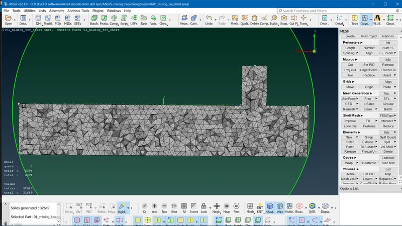
For meshing, I am using ANSA pre-processing software for any geometry cleanup and meshing of the geometry.

1. Once the geometry is opened in ANSA we select the area of interest(geometry extraction). Since this is an internal flow problem our area of interest is internal geometry. Hence this is extracted by using the option RELEASE to select the double cons. After performing the above option the necessary geometry is kept and external geometry is deleted by using the DELETE option(PID region).
2. The next step is creating the HOT and COLD inlet and OUTLET lids using FACES=>NEW=>CONS=>SELECT THE SINGLE CONS=>OK.
3. In this step, we are creating the individual for the entire cylinder geometry using the PID option.
4. Finally, once the geometry is obtained we move on with the meshing by changing the option to MESH. First we give PARAMETERS=>LENGTH(3mm)/(7mm)==>OK. Then use MESH GENERATION option=> ADVANCE mesh=> select the geometry=>ok.
5. Once the surface meshing is done we find the inside VOLUME by using the DEFINE option then do remesh to obtain the VOLUME mesh of the mixing tree. To check whether the volume meshing is performed using the CUT PLANE option to check.
6. Finally mixing tree is done with surface meshing and volume mesh we save this file as .msh to import this file into ANSYS fluent software.

MESHED TREE MODEL(LENGTH=3mm)

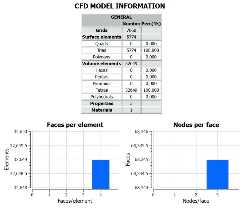
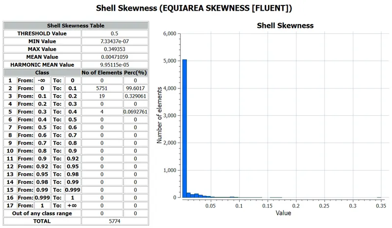
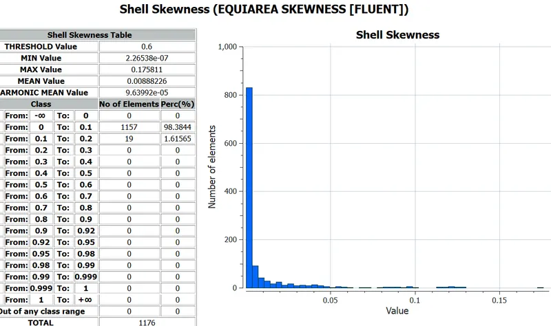
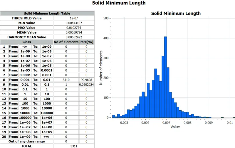
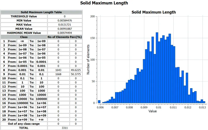
mesh quality criteria

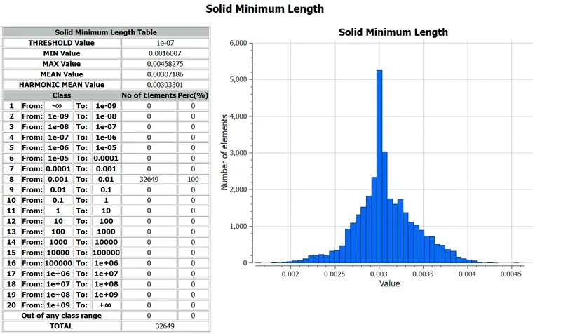
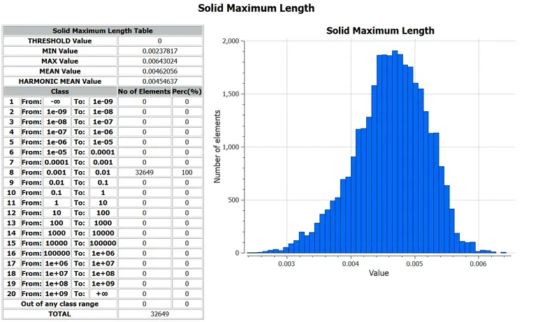
GOOGLE DRIVE FILE FOR 3mm MESHED MODEL

https://drive.google.com/file/d/1n6W5833LIC6Mv6cAYYZvnPLU88AKEmEs/view?usp=sharing

MESHED TREE MODEL(LENGTH=7mm)

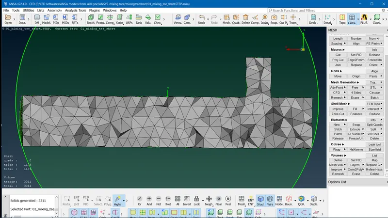
mesh quality criteria

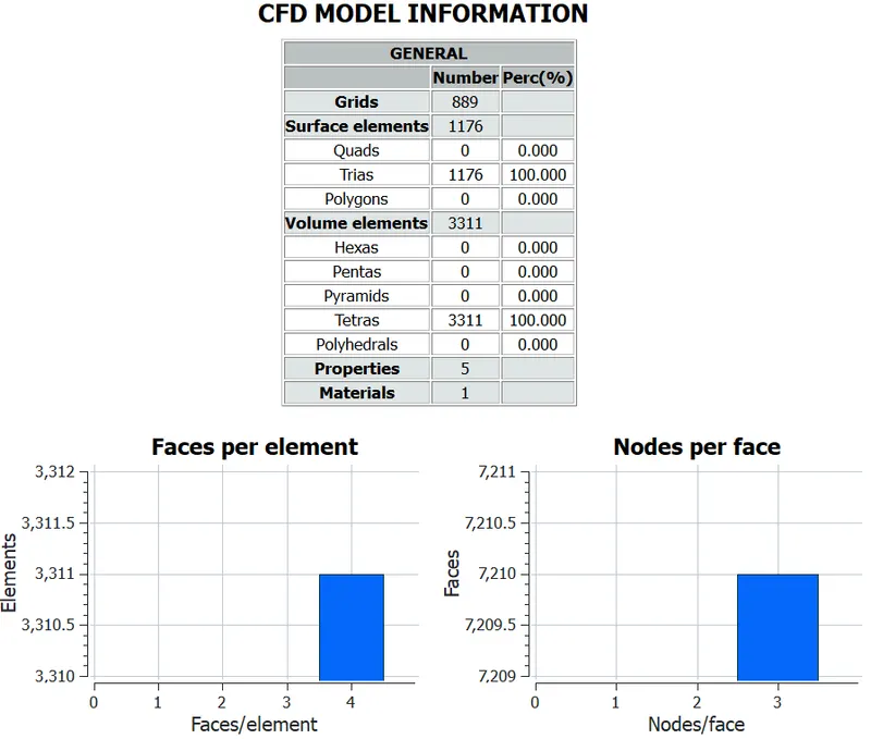
GOOGLE DRIVE FILE FOR 7mm MESHED MODEL

https://drive.google.com/file/d/1kHO_nUdqChhaf3ZApnDPKWZ3cMjhD01r/view?usp=sharing

ANSYS FLUENT

In ANSYS fluent we are studying the mixing tree model for two different mesh element sizes (3mm and 7mm) to analyze the mixing tree model to get optimum results for a series of simulations.

BASIC STEPS TO BE FOLLOWED IN ANSYS TO PERFORM SIMULATION

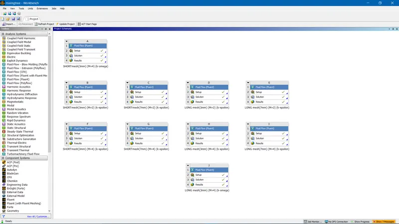
1. First, we open the ANSYS workbench we get blank space, so we create FLUID FLOW fluent on the workbench. Once this is done we get SETUP, SOLUTION, and RESULTS.
2. In the following step, we import the mixing tree.msh file into SETUP MODEL of the FLUID FLOW fluent on a workbench.
3. Once we open the SETUP MODEL the surface and volume meshed tree model opens up. In this, we provide basic physics, types of solver, boundary conditions, and type of turbulent model used.
4. Initially, we go for the SOLVER option here we are the type of solver used is PRESSURE BASED SOLVER (M<0.3), and since the variable is not varying with respect to time select the STEADY STATE option.
5. In the following step in the PHYSICS, the window selects the VISCOUS option we get the window opened up. Here we are selecting the type of turbulence which is the K-EPSILON/K-OMEGA model check for other parameters and OK.
6. In this, we are giving the BOUNDARY conditions for the inlet hot and the inlet cold which are their respective velocity and temperatures.
7. Once this is done we go under the solution option and use INITIALIZE option to assign the above conditions and compute the model for 500 iterations. Finally, we wait for the results to be converged(same solution).
8. Note that SOLUTION and SETUP windows are the same we can compute the results from the solution window. But for our convenience, we open the RESULTS window to obtain the solution to the mixing tree model.
9. Once the RESULTS window is opened we select the PLANE option to obtain the temperature and velocity at the midsection of the model and do an XY PLANE cut.
10. Then for obtaining the contour plot for variation of temperature and pressure across the length, Under PLANE we do a COLOR option to change the VARIABLE option to temperature. Similarly, these steps are repeated for velocity and pressure contour.

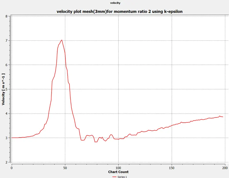
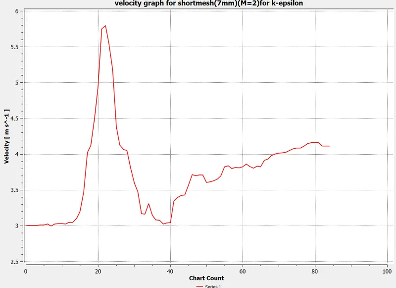
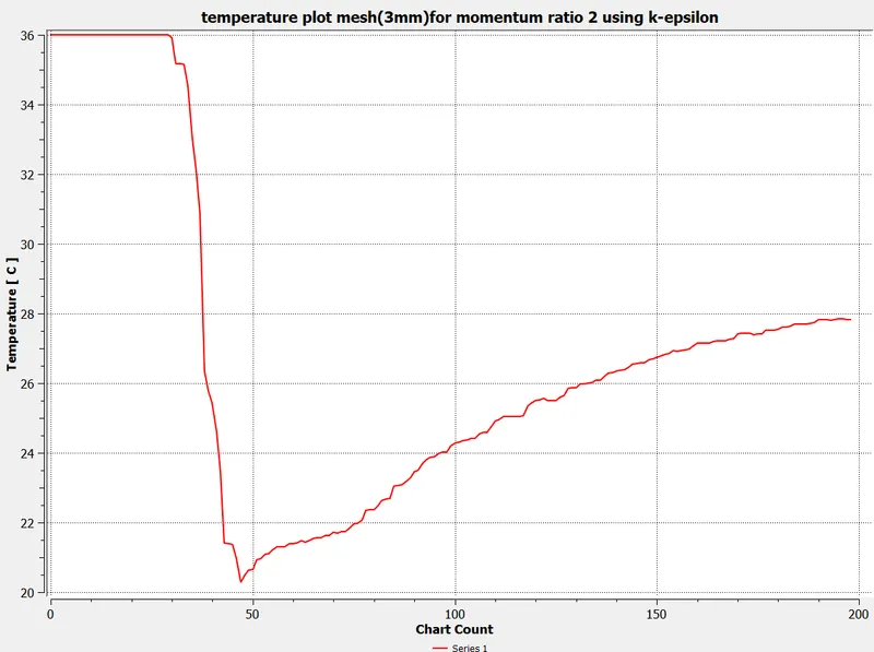
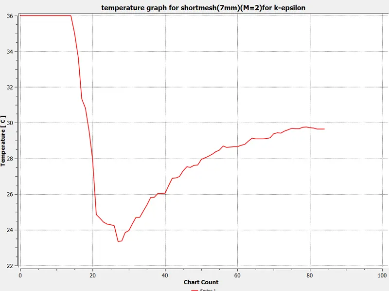
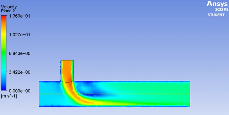
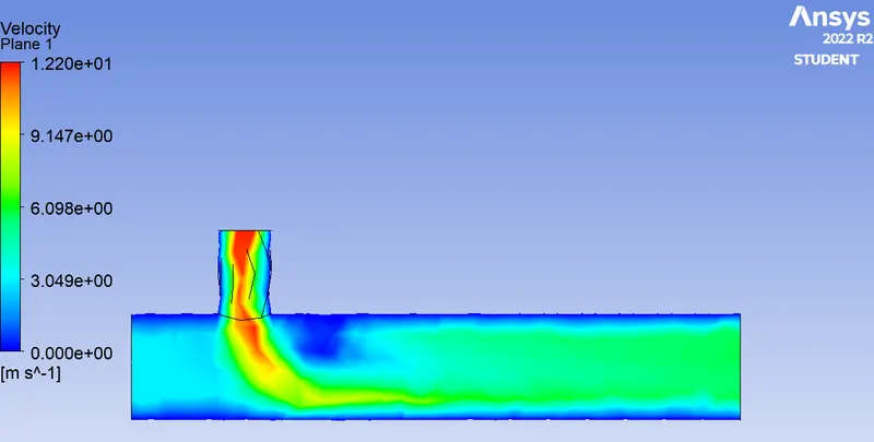
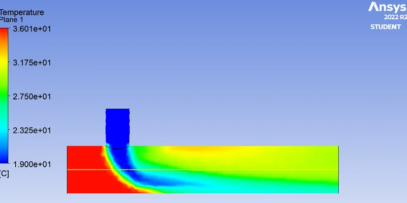
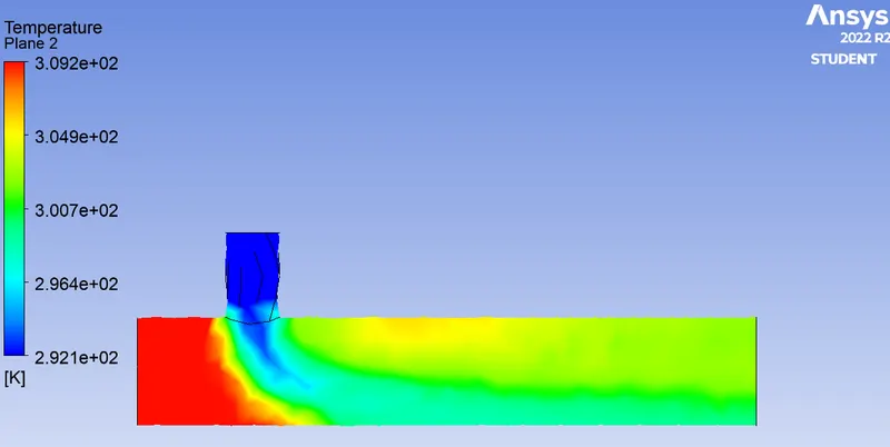
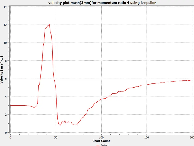
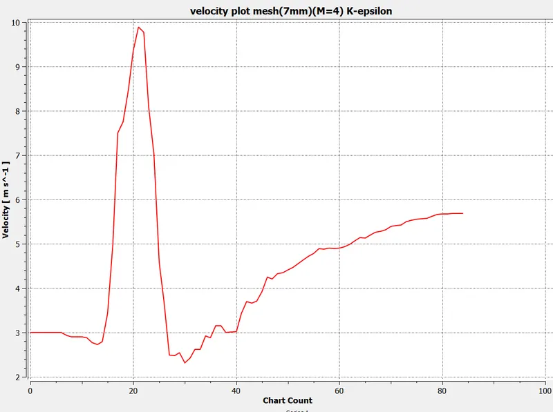
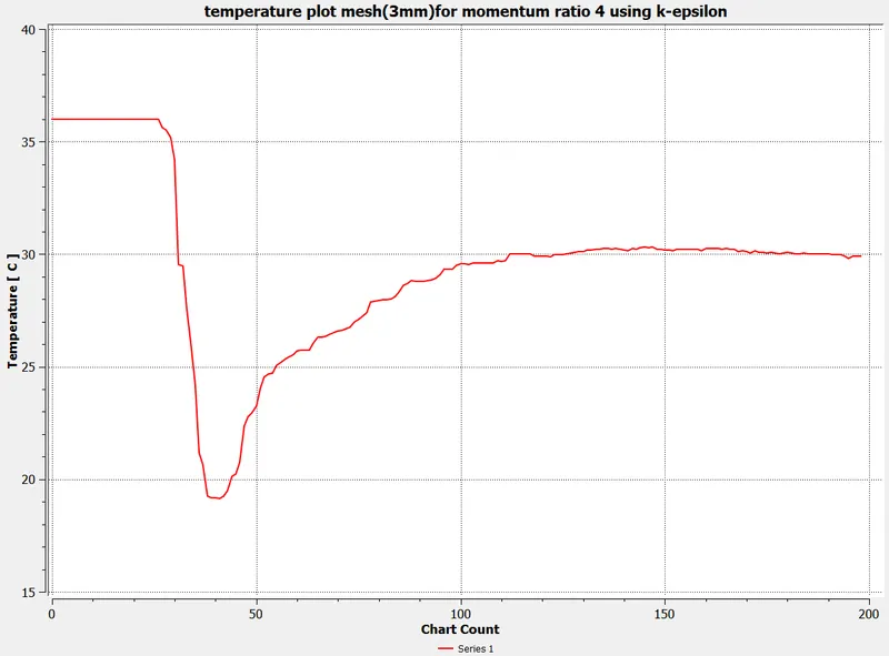
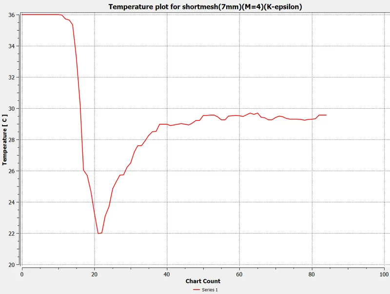
Let's compare the results for SHORT MIXING TREE using the K-epsilon model for different mesh sizes and momentum ratio

MESH SIZE=3mm(M=2) MESH SIZE=7mm(M=2)

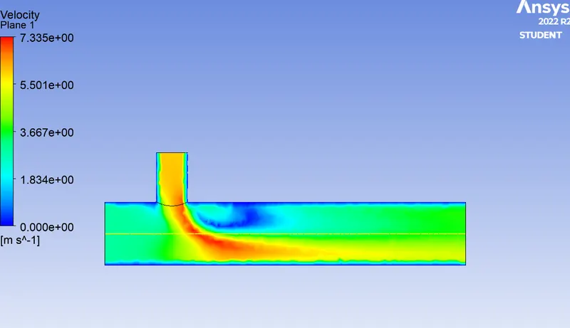
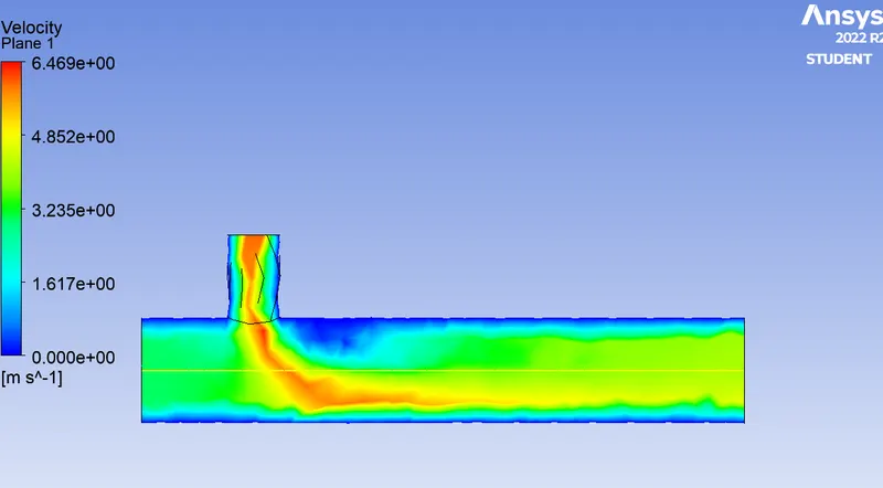
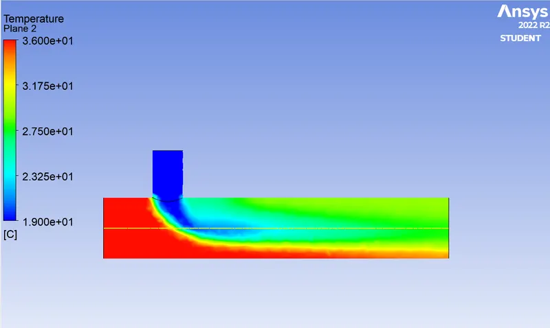
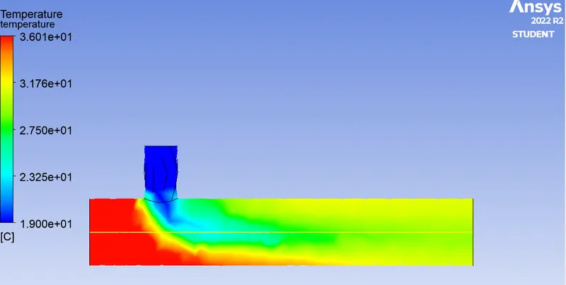
MESH SIZE=3mm(M=4) MESH SIZE=7mm(M=4)

SHORT MIXING TREE using the K-omega model

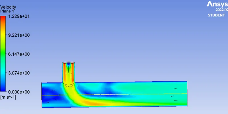
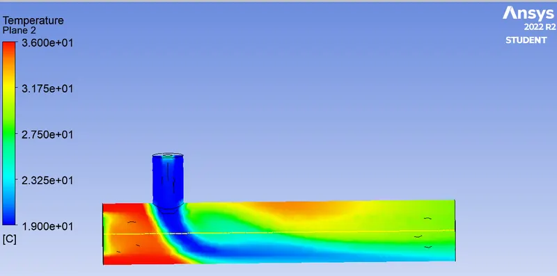
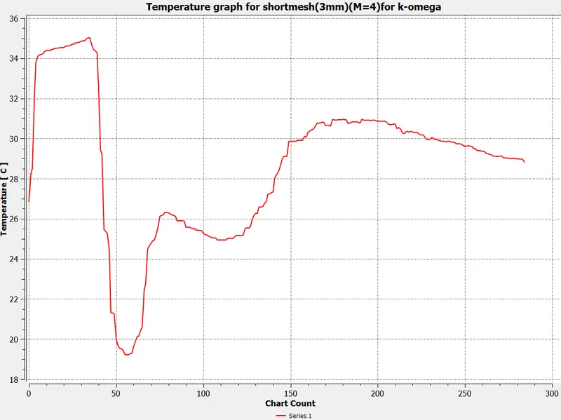
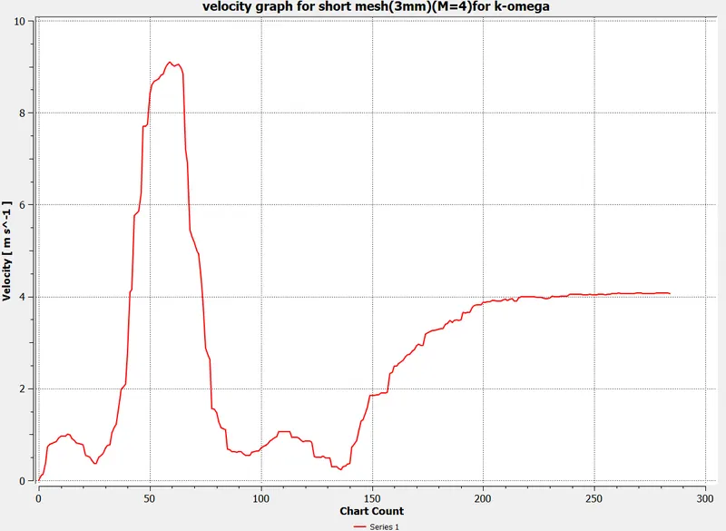
	MR=2	MR=2	MR=4	MR=4
ELEMENT SIZE	OUTLET TEMPERATURE(C)	STANDARD DEV	OUTLET TEMPERATURE(C)	STANDARD DEV
7mm	29.64	1.52	29.56	2.15
3mm	29	1.96	29.9	1.98

	MR=2	MR=2	MR=4	MR=4
ELEMENT SIZE	OUTLET VELOCITY(m/s)	STANDARD DEV	OUTLET VELOCITY(m/s)	STANDARD DEV
7mm	4.12	0.5	5.69	0.65
3mm	3.936	0.96	5.79	1.2

CASE STUDY 2:

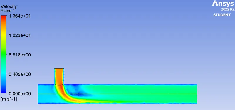
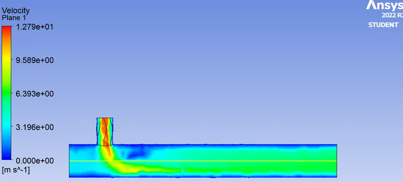
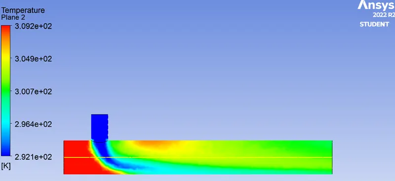
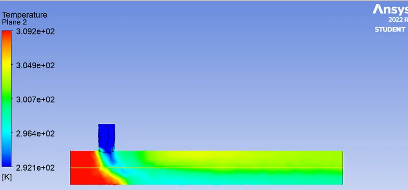
PERFORMING THE ANALYSIS ON THE LONG MIXING TREE PIPE WITH DIFFERENT MESH ELEMENT SIZES AND COMPARING THE RESULT k-EPLSION AND k-OMEGA MODEL

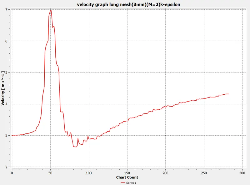
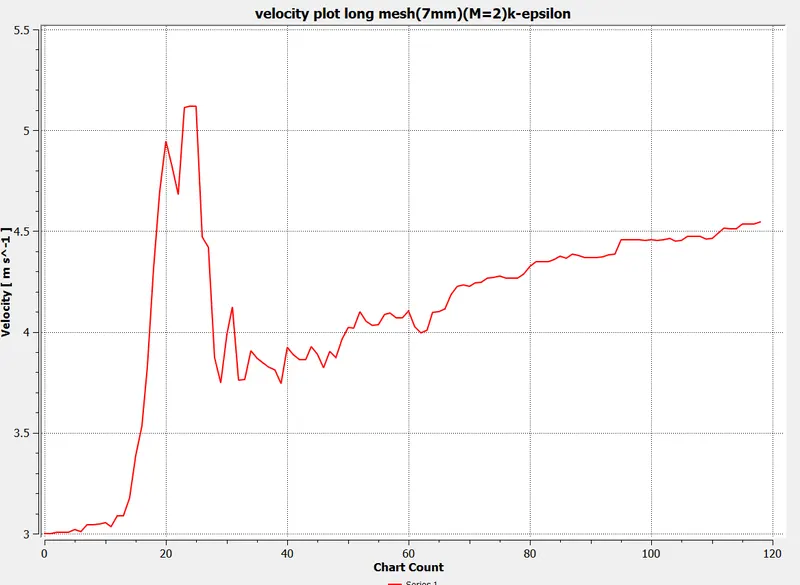
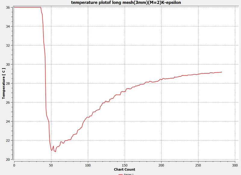
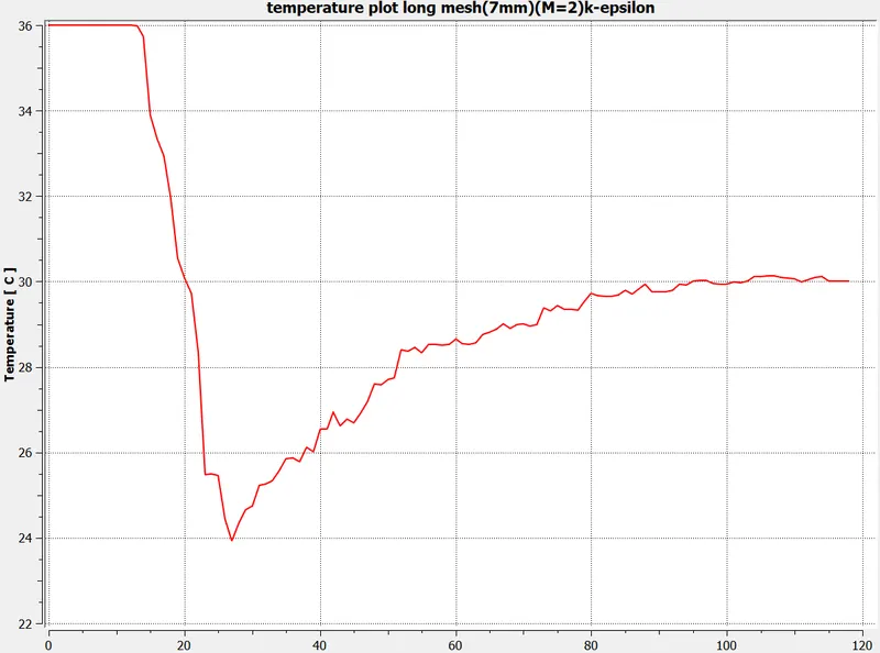
MESH SIZE=3mm(M=2) MESH SIZE=7mm(M=2)

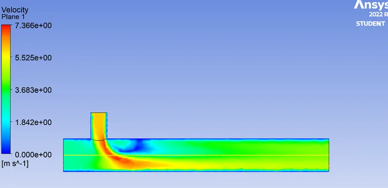
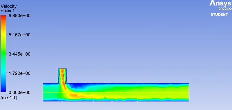
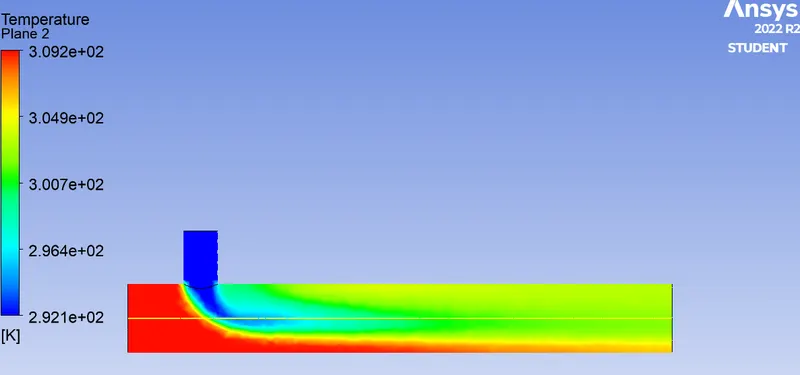
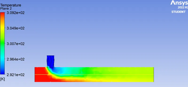
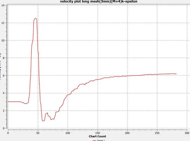
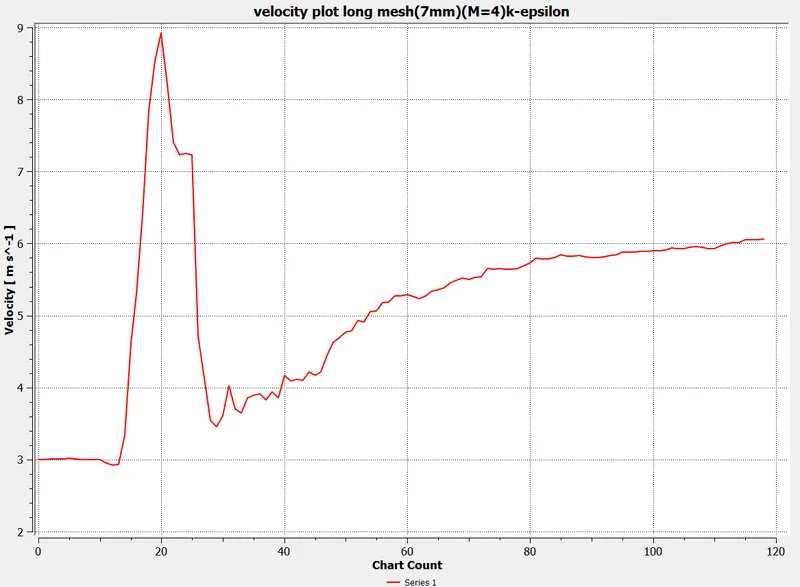
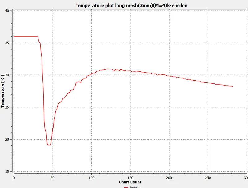
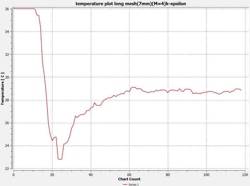
MESH SIZE=3mm(M=4) MESH SIZE=7mm(M=4)

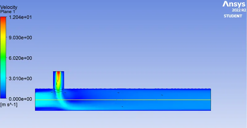
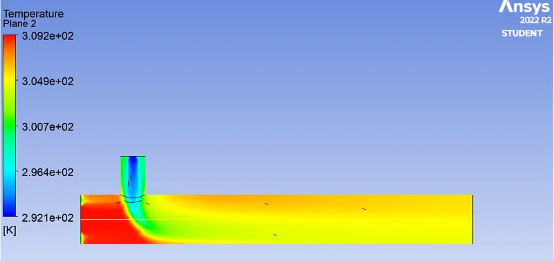
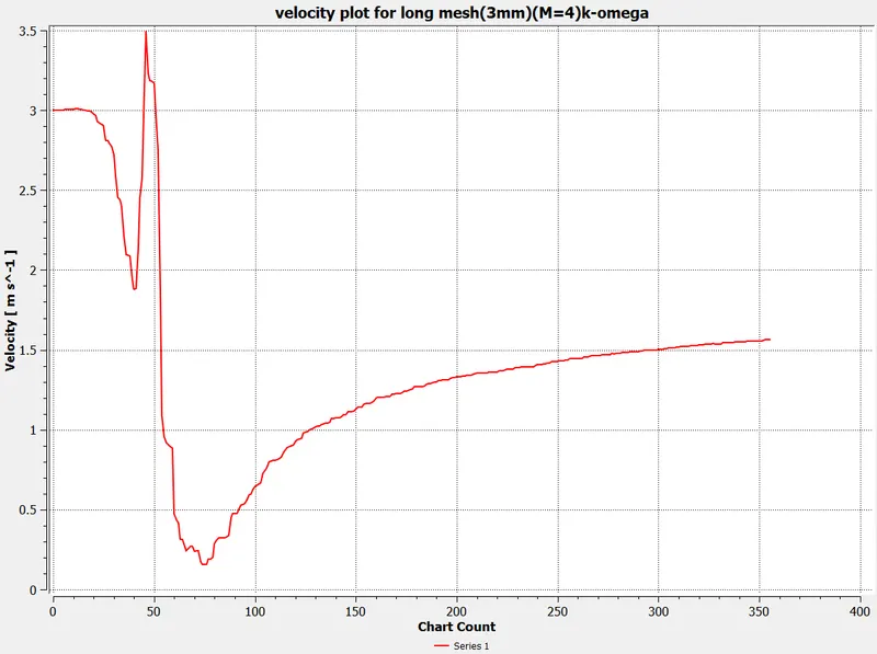
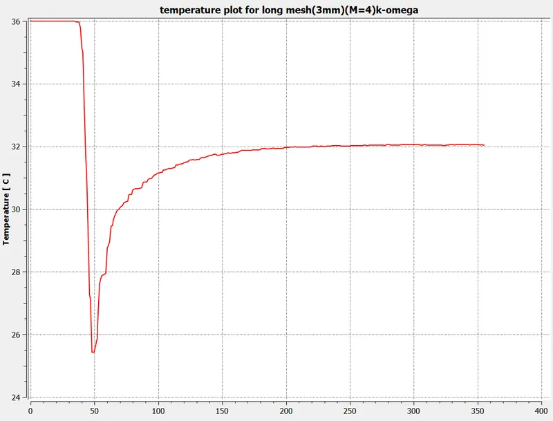
LONG MIXING TREE using the K-omega model

	MR=2	MR=2	MR=4	MR=4
ELEMENT SIZE	OUTLET TEMPERATURE(C)	STANDARD DEV	OUTLET TEMPERATURE(C)	STANDARD DEV
7mm	30.01	1.5	28.9	1.9
3mm	29.15	1.8	28.16	1.76

	MR=2	MR=2	MR=4	MR=4
ELEMENT SIZE	OUTLET VELOCITY(m/s)	STANDARD DEV	OUTLET VELOCITY(m/s)	STANDARD DEV
7mm	4.522	0.65	6.05	0.8
3mm	4.31	0.55	6.175	0.9

DRIVE LINK ANSYS FLUENT MIXING TREE MODEL

https://drive.google.com/file/d/10ChZQXltm2fDAeYYJFTZuCOdRx-JjzgW/view?usp=sharing

OBSERVATIONS SHORT MIXING TREE MODEL:

• Decreasing the meshing size increases the overall element count and finer mesh or increasing mesh element size we course mesh(the results obtained in finner mesh are more absolute(accurate mixing) compared to course mesh).
• K-omega model produced a higher standard deviation which means less accuracy in predicting results for this model. So, it is recommended to use the k-epsilon turbulence model for solving this problem.
• The k-epsilon model is used to study the phenomena which are away from the wall whereas K-omega is used for studying the phenomena toward the wall.
• For the short pipe, the convergence is achieved at 150 iterations out of 500 iterations.
• Higher the momentum ratio hence the amount of cold fluid entering the pipe also be higher due to the there higher relative velocity between the fluids hence it experiences higher turbulence. Thereby outlet temperature decreases which indicate a higher momentum ratio hence efficiency is higher.
• The finer the mesh higher the standard deviation of outlet velocity and the lower the standard deviation of outlet fluid temperature which infers that such fluid holds better turbulence behavior which is desired to benefit the usage of the short mixing tree model.

OBSERVATIONS LONG MIXING TREE MODEL:

From the above results, it can be assessed using a long pipe doesn’t serve the purpose efficiently since outlet fluid parameters are similar to a short pipe.

CONCLUSIONS:

1. Short-pipe at a higher momentum ratio has higher mixing efficiency.
2. It is recommended to use the k-EPSILON turbulence model since it is predicting the results very accurately.
3. An increase in the length of the pipe doesn’t serve the mixing purpose efficiently.
4. k-OMEGA model is preferred for studying near-wall conditions.