Week 1- Mixing Tee

Objective :- To set up steady-state simulations to compare the mixing effectiveness when hot inlet temperature is 36⁰C & the Cold inlet is at 19⁰C.

Use the k-epsilon and k-omega SST model for the first case and based on your judgment use the more suitable model for further cases. Giving the reason for choosing a suitable model is compulsory.

1. Case 1
   • Short mixing tee with a hot inlet velocity of 3m/s.
   • Momentum ratio of 2, 4.
2. Case 2
   • Long mixing tee with a hot inlet velocity of 3m/s.
   • Momentum ratio of 2, 4.

In a table, compare the following values from the 2 cases.

1. Cell count
2. Average outlet temperature
3. Number of iterations for convergence

Expected results:

1. Velocity and temperature contour plots on the cut planes along and across the pipe.
2. Velocity and temperature line plots along and across the length of the pipe.
3. Perform Mesh independent study for any one case.
4. Discuss the effect of length and momentum ratio on results.

Procedure

Understand k-epsilon and k-omega SST by considering case-1

Let us start with analyzing the best method to converge the solution for this particular case by studying two methods: k-epsilon and k-omega SST.

In this study will set two setups, one for k-epsilon and another for k-omega SST. Here, we are going to use the same geometry and mesh for both cases of simulation. Hence, we are going to use a short mixing tee model

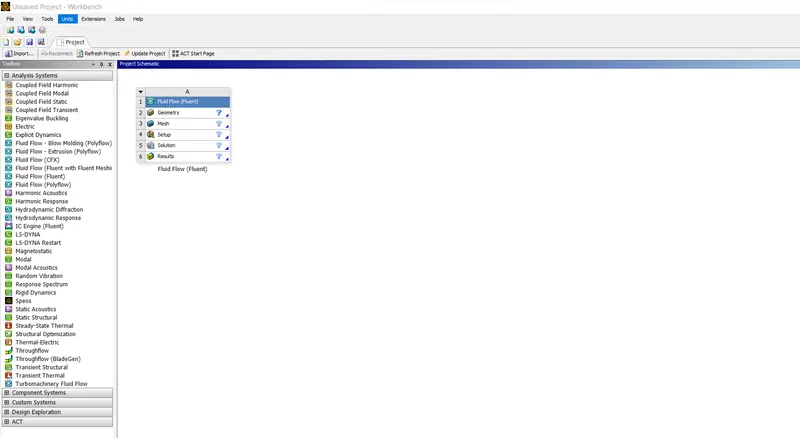
1.Open new project, by clicking on Fluid flow (Fluent) in Ansys workbench.

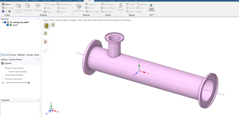
2. Now click on geometry to import mixing tee model and extract the fluid volume (working fluid volume) using volume extract option in prepare tools.

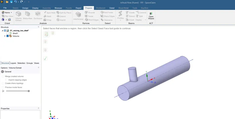
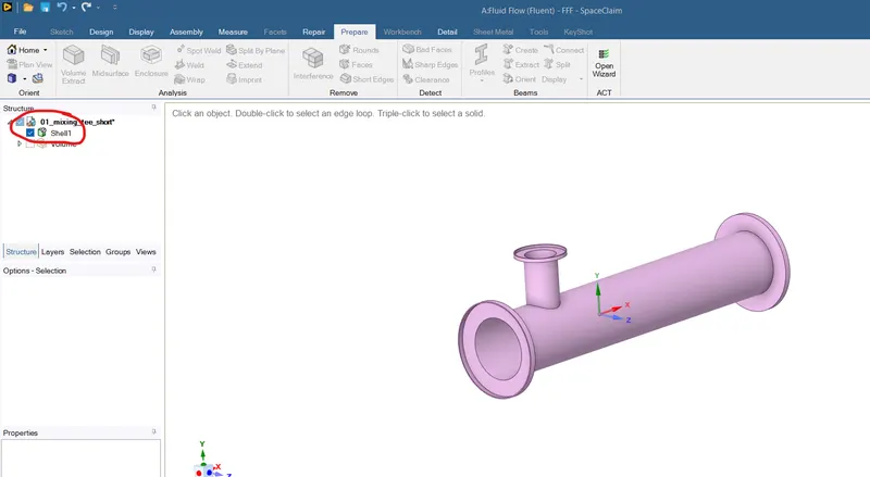
3.Suppress the actual model, as we do not have to make any conduction simulation in this project. Lastly, close the space Claim.

4.Now, we can go for meshing. So, click on the mesh button, which will start Ansys meshing, where we can generate the mesh and provide names for all the surface of the geometry.

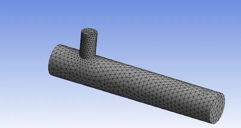
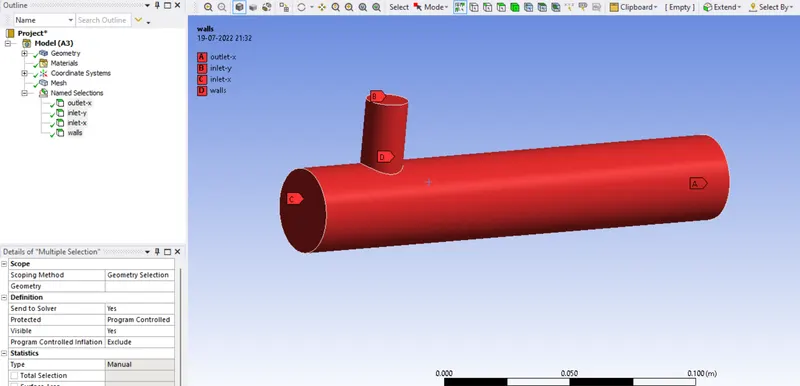
5. Select the option element quality to see, how many elements are defying quality. Quality is measured on the scale of 0 to 1. In our graph most of the element are near to 1 so we can say it is good quality.

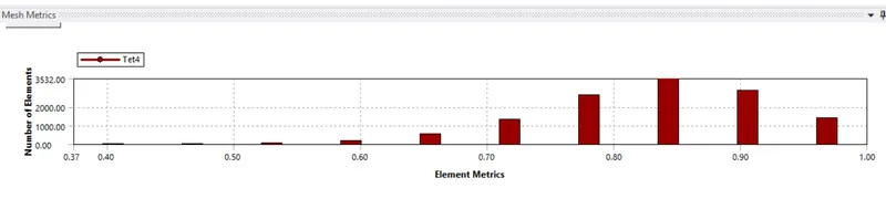
from the above graph we can say that few elements are falling in 40% (0.40) quality range so it is acceptable and good mesh, if any elements falling in 5% (0.05) range then the mesh is failing for quality.

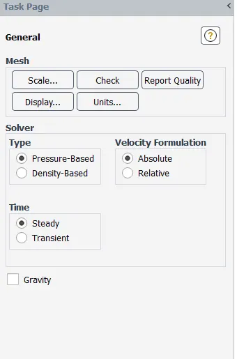
6. Exit mesh and open setup. First, Check mesh, it is throwing no error then only we can proceed further. We are going to do pressure based steady state simulation, so choose these options on task page.

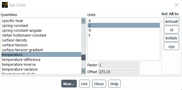
7. Click ‘units’ to change the units of temperature. FLUENT store values in SI units. Most post-processing can be converted into other units.

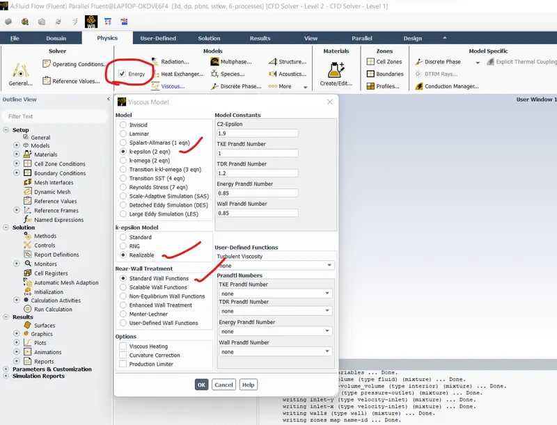
8. Go to physics menu and Turn on the energy Equation. Activating energy equation allows the temperature-dependent problem to be solved. In the viscus model, select ‘k-epsilon’,’ Realizable’ for our first type of simulation. Turbulence modeling is a complex area. The choice of model depends on the application. Here, the Realizable k-epsilon model is used which is an improvement on the well-established standard k-epsilon model. Accept the remaining default settings.

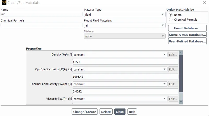
9.In materials click “FLUENT Database’ to add new material. In this case, our working fluid is air so we keep the default material.

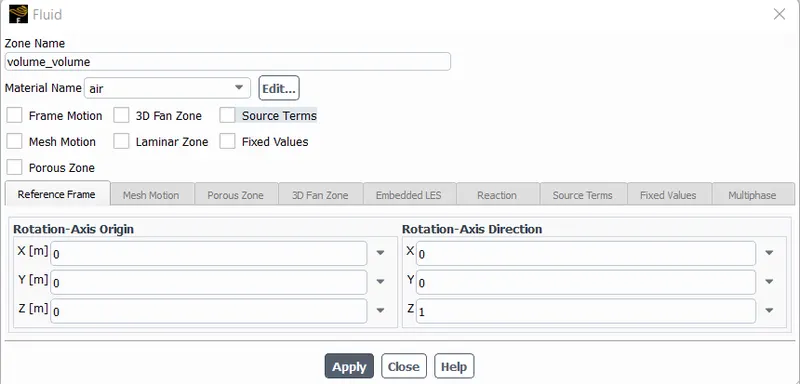
10. In the cell zone define the material, select the working fluid.

Boundary conditions

11. In ‘Boundary condition’ click on the ‘Inlet-x’ and edit the inlet parameter set velocity as 3m/s and temperature as 36^oC. For inlet_y set velocity as 12m/s as we are using momentum ratio of 4 and temperature as 19^oC.

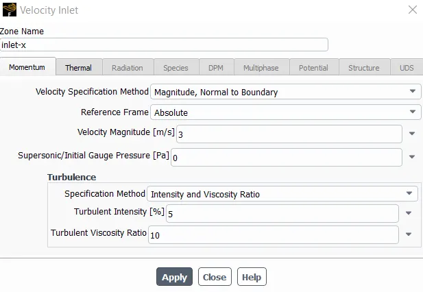
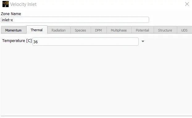
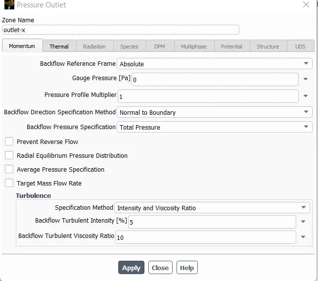
Set outlet pressure condition as atmospheric pressure value which is also zero gauge pressure. The simulation may predict that flow enters the model through part of the outlet. The backflow will bring turbulence and energy back into the model. However, the model can not predict how much (because the flow is coming from outside of the model). It is, therefore, necessary to specify backflow conditions. Ideally, the geometry should be selected such that flow enters the model only at well-defined inlets. The backflow setting then does not affect the final solution (although they may be used in intermediate iterations).

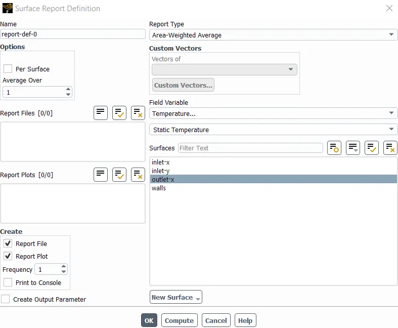
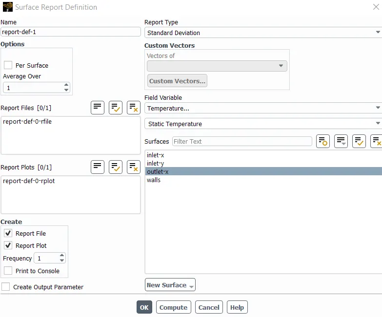
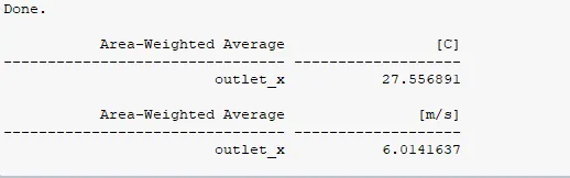
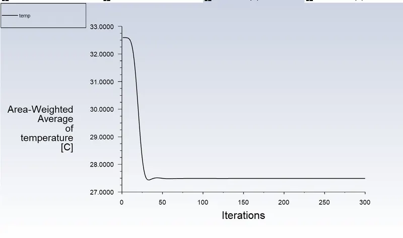
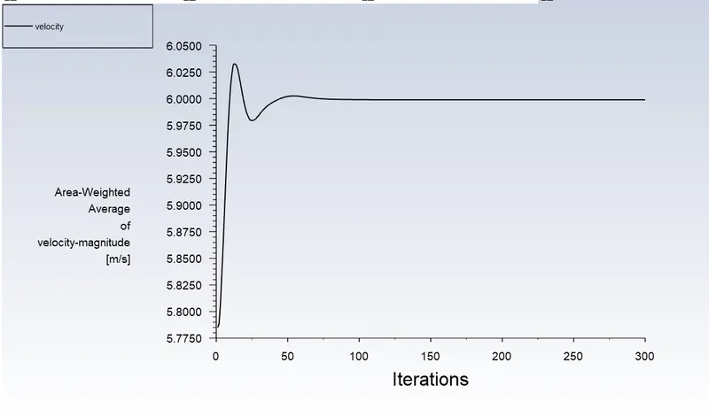
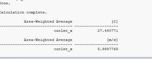
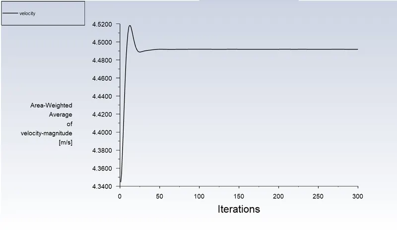
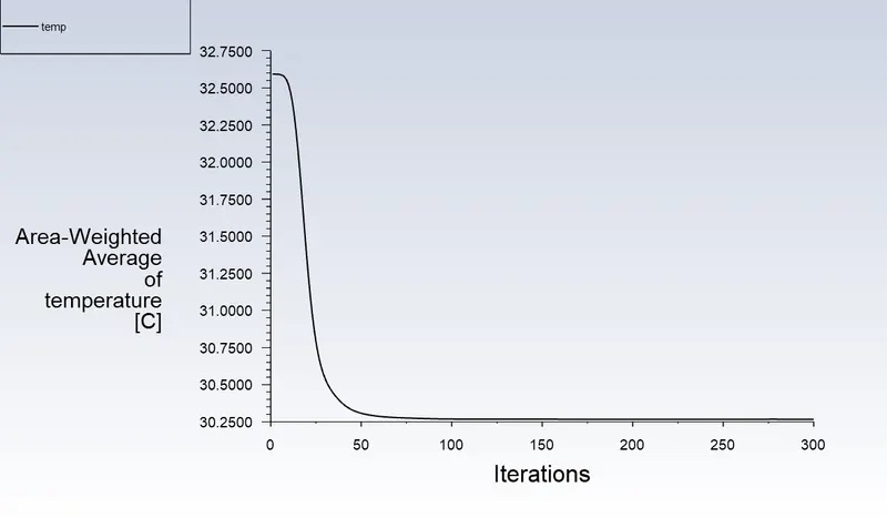
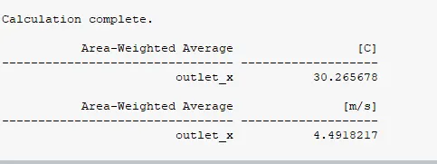
12. go to Solution - ‘Reports’, press ‘new’ for the surface report monitor. Select area-weighted average. Here we want temperature average at outlet surface and standard deviation of temperature also.so select temperature as field variable And check “report file” and “report Plot”.

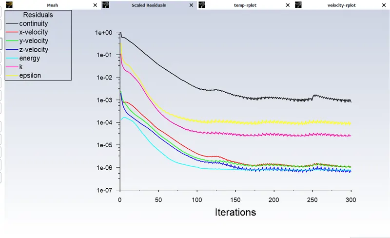
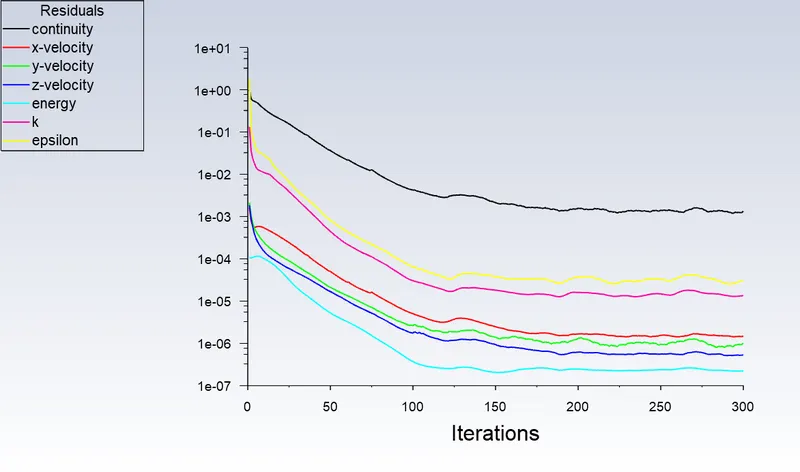
13. Now click on hybrid initialization . Change the number of iterations to 300 and click on calculate. If solution is not converged, then iterations can be increased.

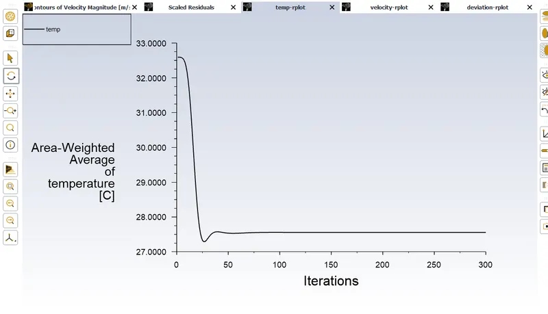
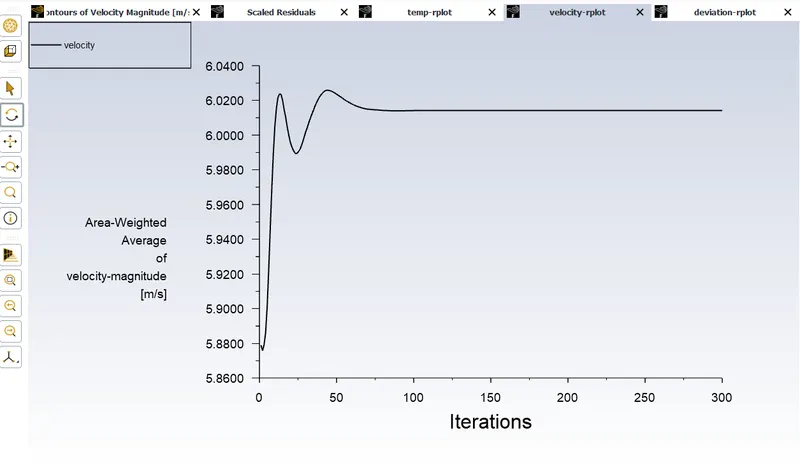
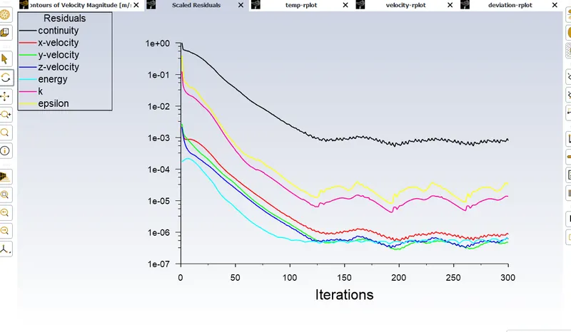
While calculating the solution we will also get our converge plot for the k-epsilon method. It also built up another plot report of temperature and velocity at the outlet that we set earlier

After this, we can close the fluent and post-process the results. Click on the results in the workbench and it will open CFD-Post.

CFD-Post initially displays the outline (wireframe) of the model which can be turned on by checking the surface shown in the Outline panel in the fluid section.

Viewer toolbar buttons allow you to manipulate the view.

Create a plane - in the location menu, select ‘Plane’ -> accept the default name ‘Plane 1’ -> set ‘Method’ to be ‘YZ Plane’, accept ‘X’ as 0.0, and press ‘Apply’

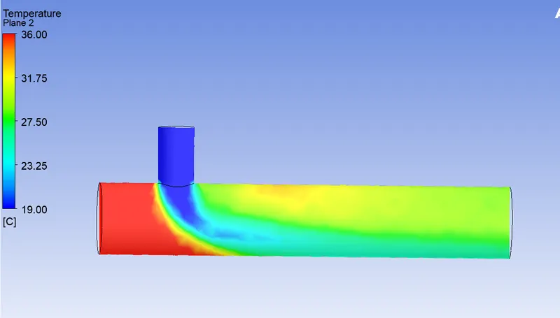
Finally, select a plane from the Outline section and use color by temperature which will generate temperature contour on the selected plane.

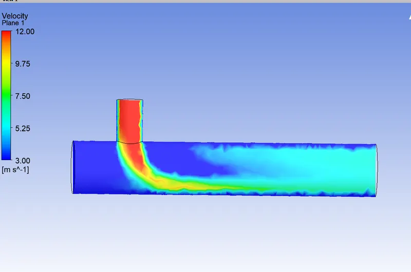
Now, create another plane for velocity contour.

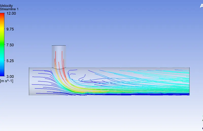
14. now we are going to use the same setting for the next simulation and solve the problem by the k-omega SST method. And compare all the results

For the k-omega SST method

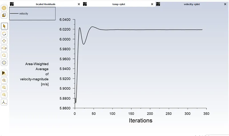
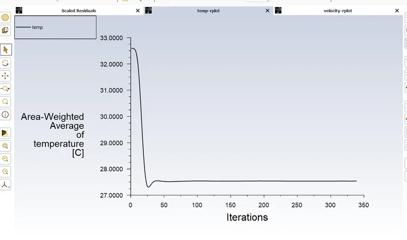
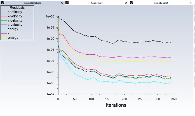
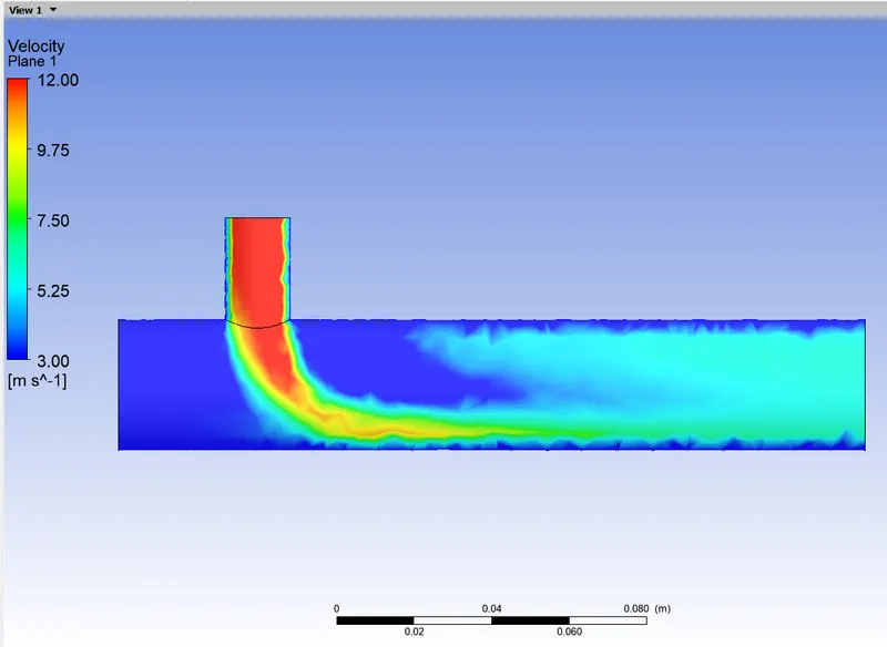
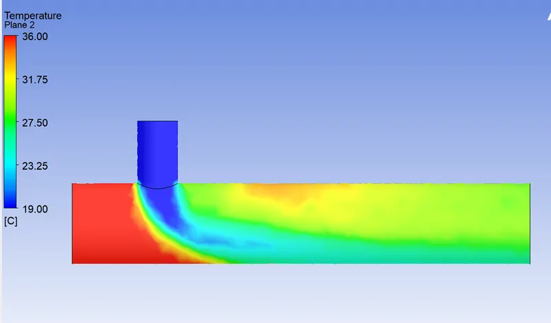
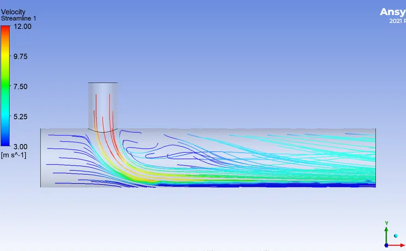
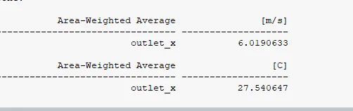
k-Epsilon

- as we saw in our first simulation, the K-epsilon turbulence model is the most common model used in CFD to simulate mean flow characteristics for turbulent flow conditions. It is a two-equation model that gives a description of turbulence by means of two transport equations (PDEs). the first transported variables are the turbulent kinetic energy (k) and the second transported variable is the rate of dissipation of turbulent kinetic energy.

k-epsilon focuses on the mechanism that affects the turbulent kinetic energy.

k-omega SST

The SST k-omega turbulence model is a two-equation eddy-viscosity model that is used for many aerodynamic applications. It is a hybrid model combining the Wilcox k-omega and the k-epsilon models. A blending function, F1, activates the Wilcox model near the wall and the k-epsilon model in the free stream. This ensures that the appropriate model is utilized through the flow field

Main difference

The k- omega model is well suited for simulating flow in the viscous sub-layer. On the contrary, The k-epsilon model is ideal for predicting flow in the regions away from the wall

The SST model exhibit less sensitivity to free stream conditions (Flow outside the boundary layer) than many other turbulence models.

The shear stress limiter helps the k-omega model avoid a build-up of excessive turbulent kinetic energy near stagnation points.

If we observe our simulated figure, we can notice, in the k-omega model flow is more like laminar and not giving proper turbulent results, in contrast, simulation by k-epsilon, is giving proper mixing of the two air stream.

In this particular case we are not dealing with walls, therefore, we are going to use the k-epsilon method for further simulations.

Case-2-a

Long mixing tee

Hot Inlet velocity - 3m/s

Temp -36c

Momentum ratio - 4

Inlet velocity of cold air = 3x4 = 12m/s

Temp - 19c

follow the same procedure as like case1

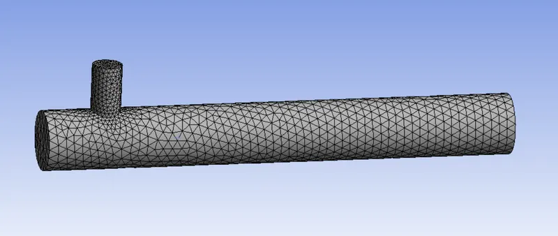
Case-2-B

Long mixing tee

Hot Inlet velocity - 3m/s

Temp -36c

Momentum ratio - 2

Inlet velocity of cold air = 3x2 = 6m/s

Temp - 19c

Conclusion:

• k-epsilon models predict flow virtually far from the boundaries (wall), and the k-omega model predicts near the wall. As in this case we need a flow simulation turbulent model far from the wall, therefore, the k-epsilon method is used.
• Solving the first simulation on the fluid domain using coarse mesh gives an initial overview of the analysis which converges results fast. As element number increases the convergence time also increases. Therefore, after obtaining the rough results using coarse mesh simulation successfully we can improve mesh quality and get to final accurate results doing this saves a lot of time which is also extremely helpful for mesh independence test.
• To get better mixing at outlet high velocity of flow is very effective. Therefore, a higher momentum ratio gives better mixing of hot and cold fluid stream at the outlet.
• As the Length of the mixing tee increases because diffusion flow always gives slightly better mixing of two-fluid.
• Finally, in the above cases, it is very important to use a short mixing tee with a momentum ratio of 4 to get precise results but one has to consider the diffusion of flow along the length of the mixing tee, a long mixing tee with momentum will be the greater option.