OBJECTIVE.
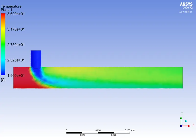
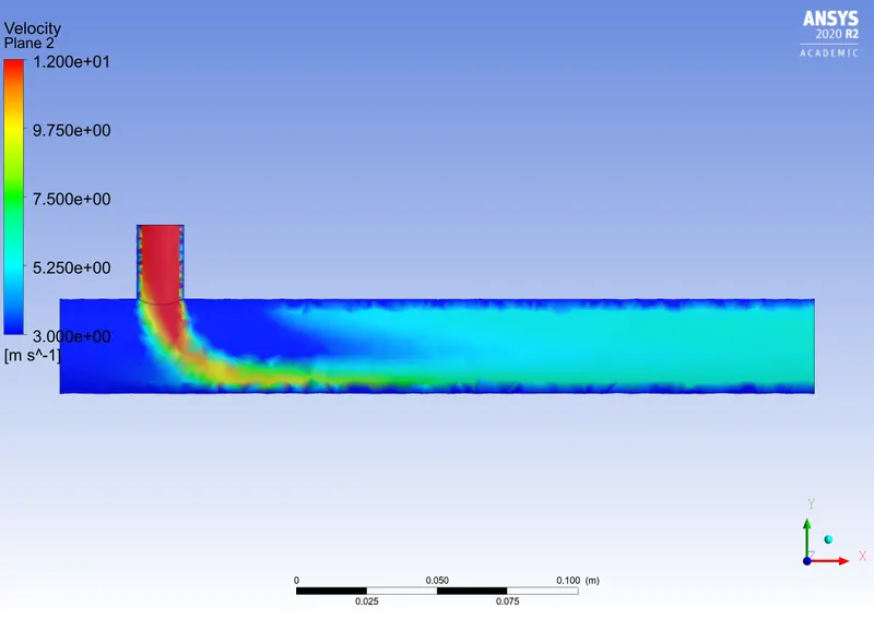
- To set up steady-state simulations to compare the mixing effectiveness when hot inlet temperature is 360C & the Cold inlet is at 190C by using the k- epsilon and k-omega SST model.
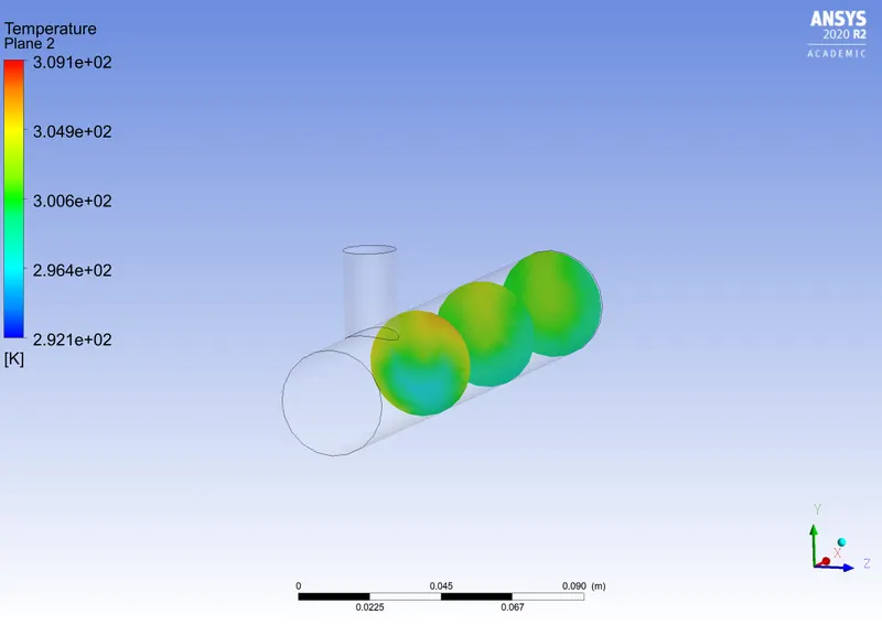
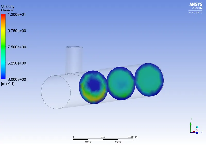
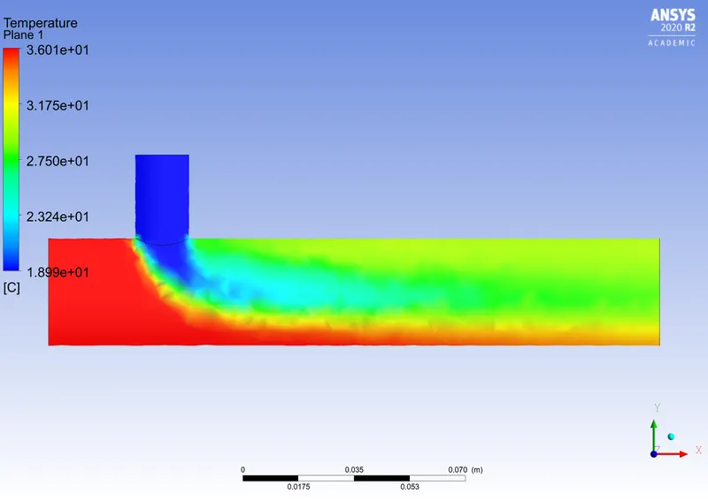
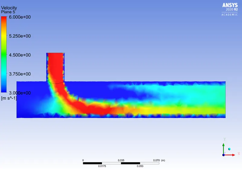
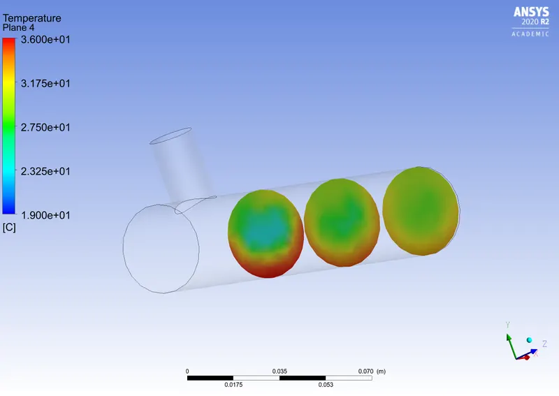
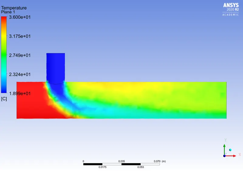
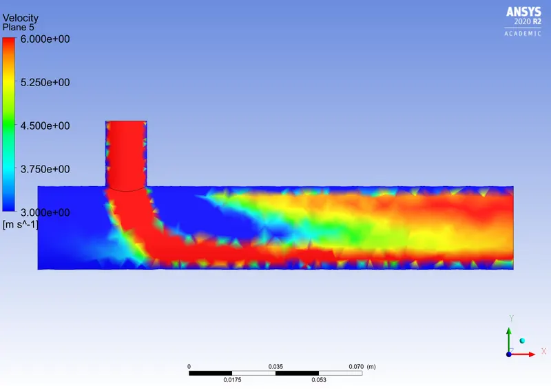
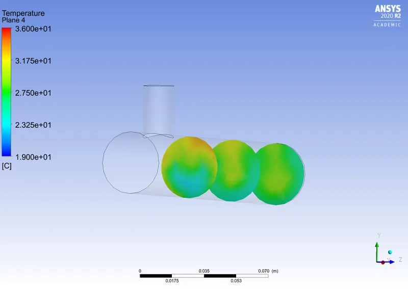
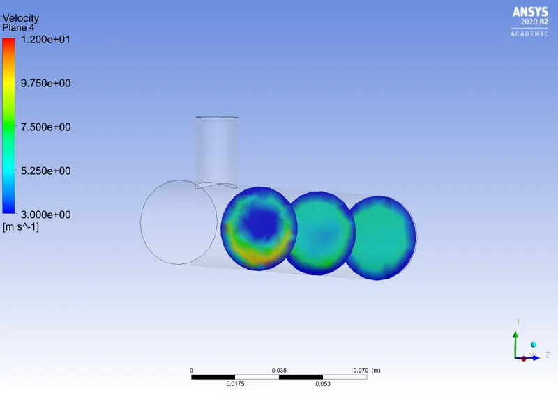
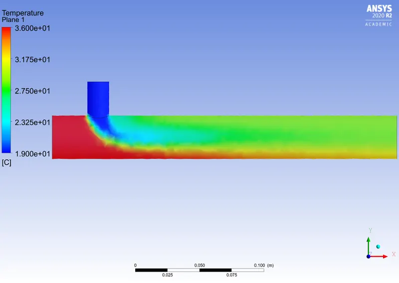
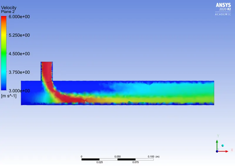
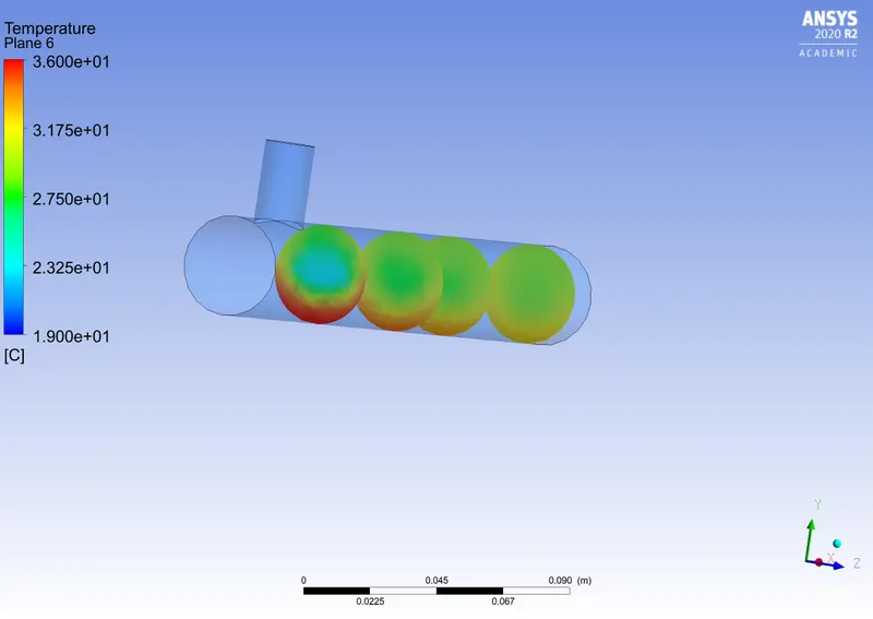
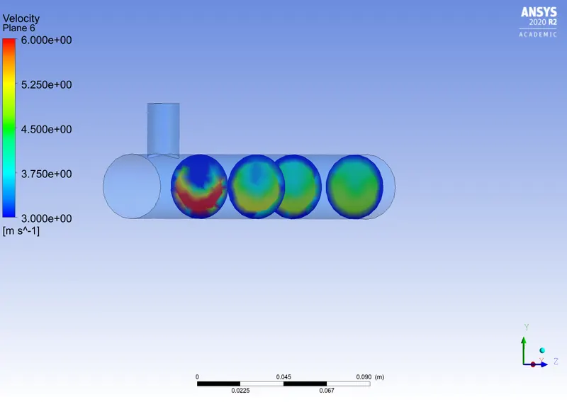
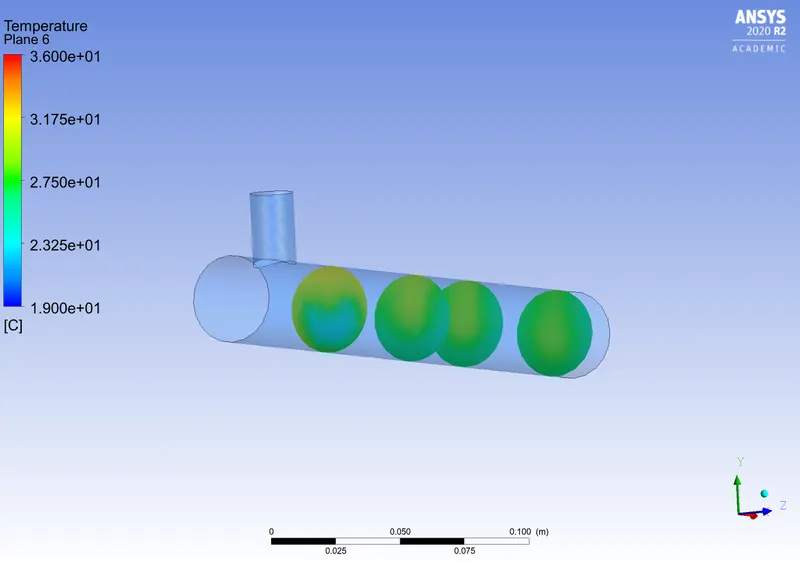
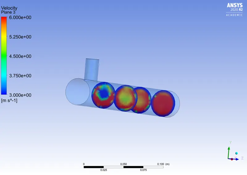
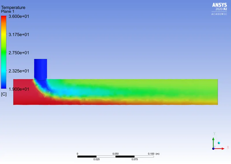
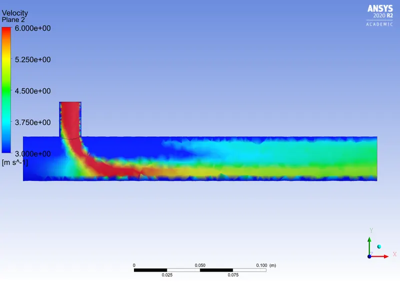
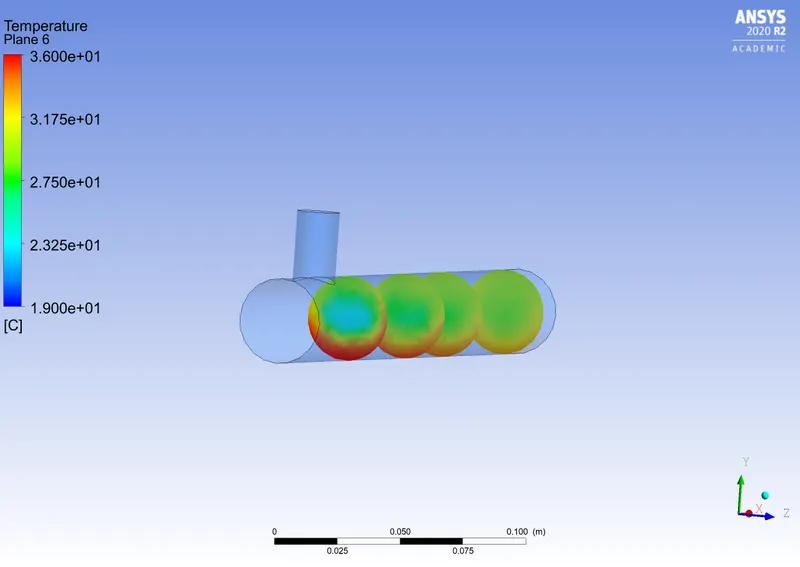
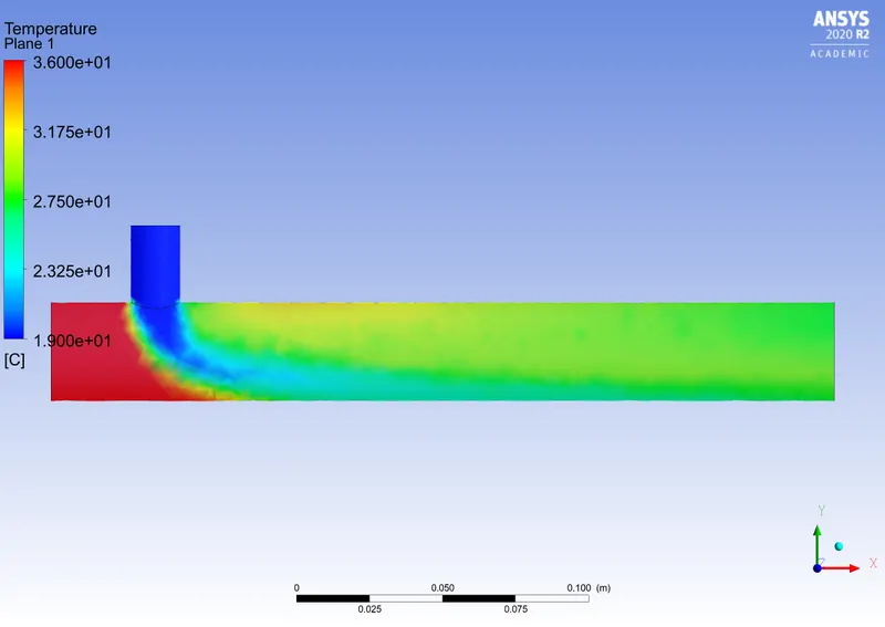
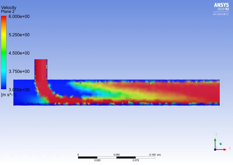
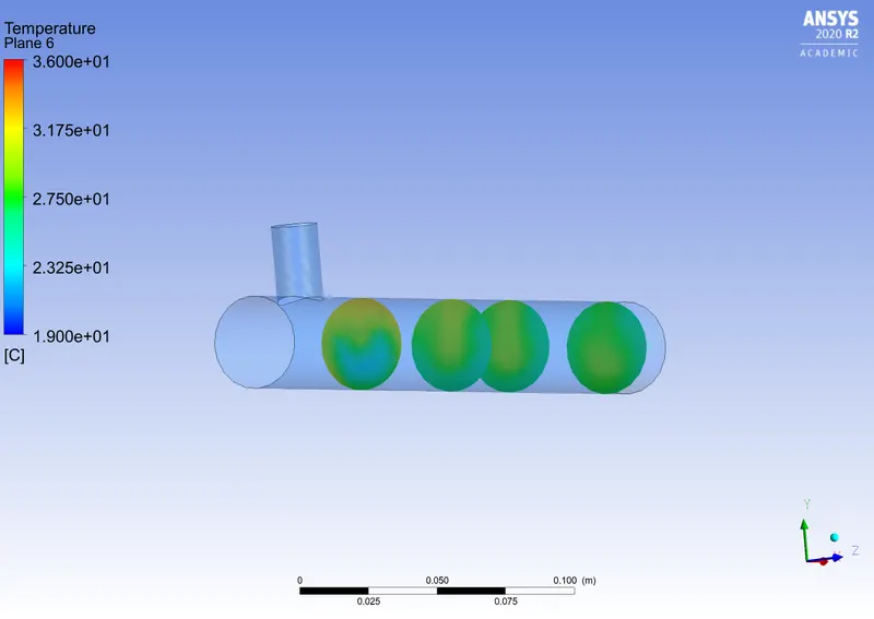
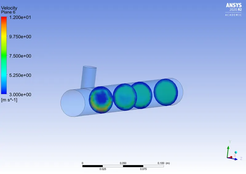
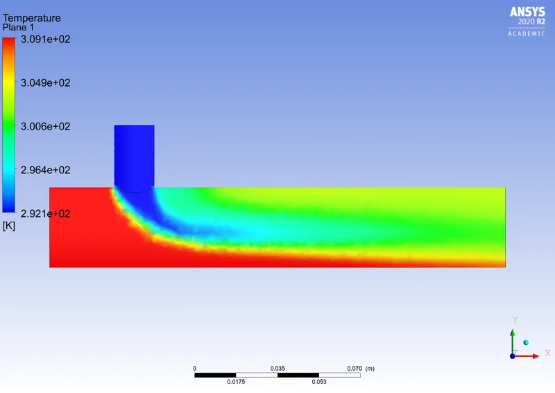
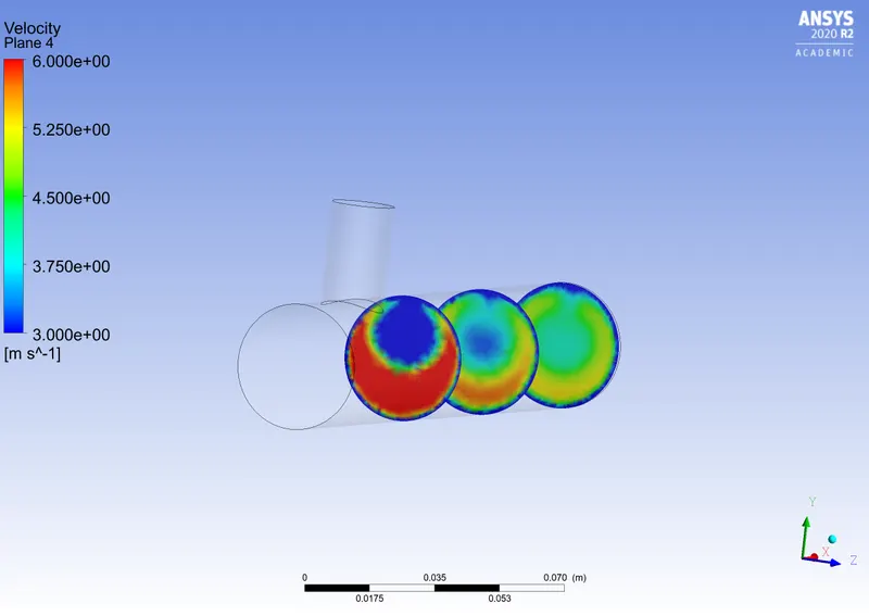
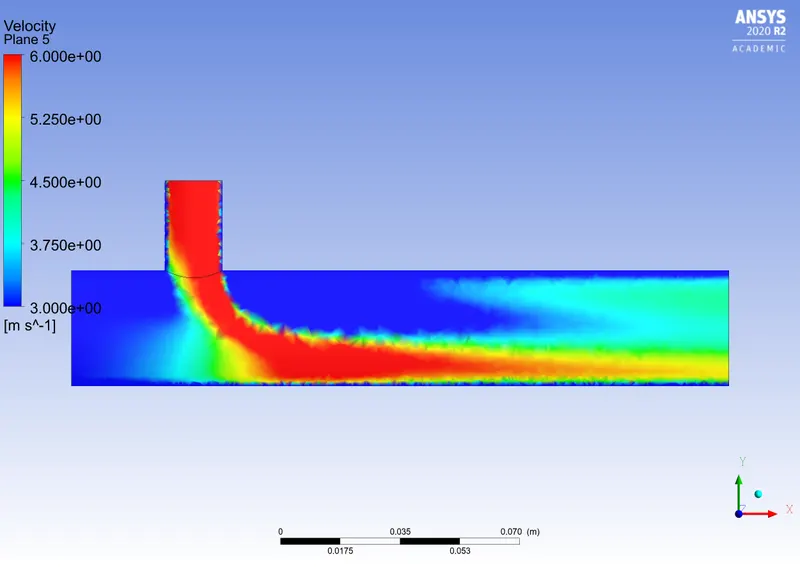
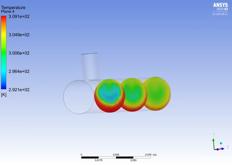
- And to plot Velocity and temperature contour plots on the cut planes along and across the pipe.
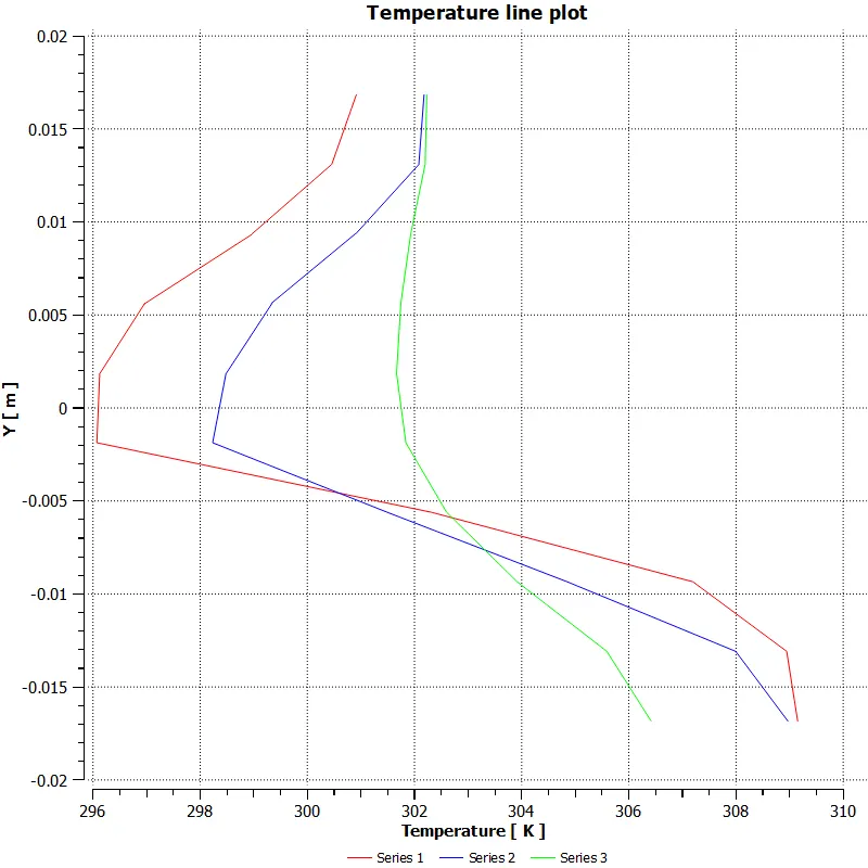
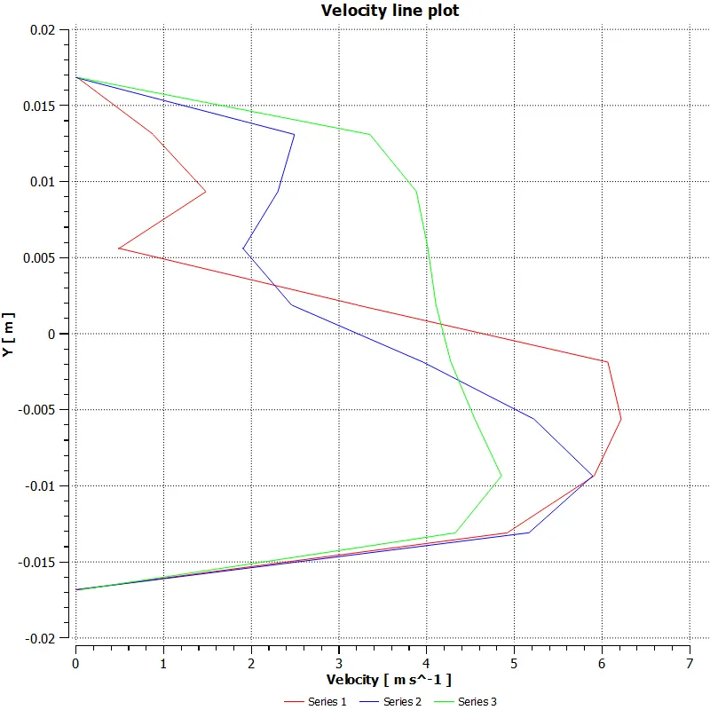
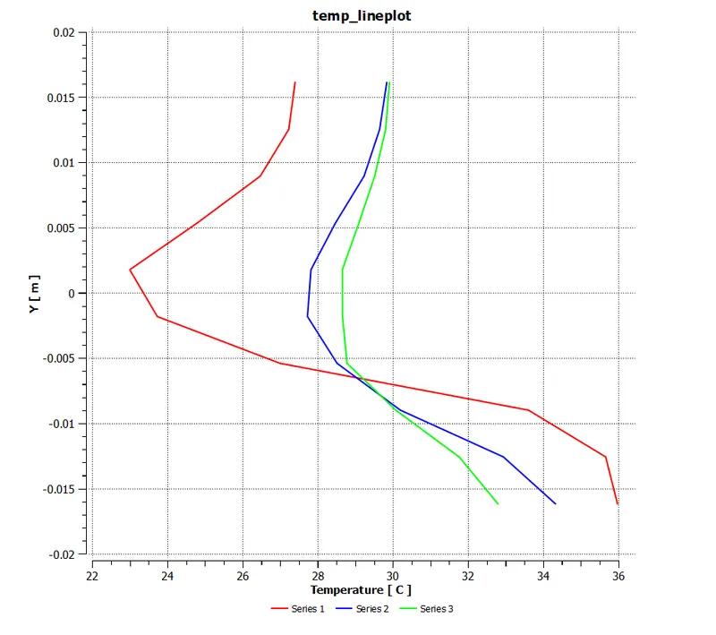
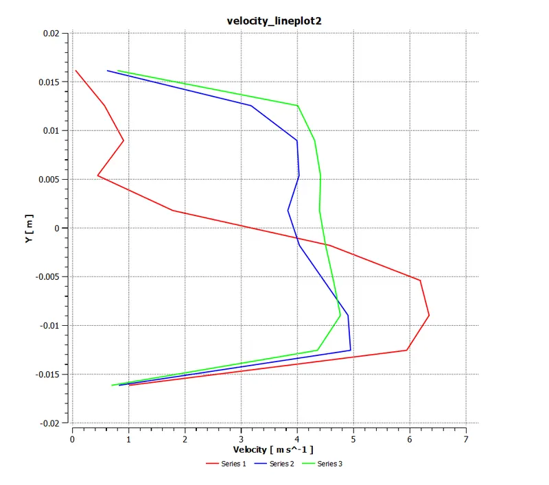
- To plot Velocity and temperature line plots along and across the length of the pipe.
- To Perform Mesh independent study for any one case.
MIXING Tee.
A tee is formed by two pipe sections joined at a right angle to each other. The hot fluid (water) is flowing through the main pipe
while the cold fluid (water) enters the main pipe through the branched pipe. There have been traditionally developed empirical
design equations to solve the mixing problems but it does not take into account the complexity of turbulent flow in applications like
petrochemical products, waste water treatment, blending of oils, etc.
With due respect to all the other industries, nuclear industry is the one where efficiency of the mixing of fluids in the mixing chambers
is very critical. There have been much of research regarding the thermal stresses arising in the T-junctions due to the large temperature
difference and also due to frequent changes in the same.
A large temperature gradient is created along the length of the pipe due to mixing of fluids near the junction as well as to the
downstream of the main pipe.
The temperature fluctuations cause cyclic thermal stresses and subsequent fatigue cracking of the pipe wall. Thus, anticipating the
failure of the piping systems in nuclear power plants is very essential as its failure may lead to irreparable damage. In order to assess
the structural strength, stability and life of such T-junctions, it is essential to know the following: (i) magnitude of the temperature
fluctuations, (ii) regions of pipe wall that experience the temperature fluctuations, (iii) response of the material of the pipe to the thermal
fatigue loading.
Noguchi et al. (2003) carried out experimental studies of thermal striping with scale models of T-junctions using hot and cold water.
They investigated the flow pattern and characteristics of the temperature fluctuations with the help of flow visualization and temperature
fluctuation measurements. They concluded that velocity ratio determines the flow pattern and temperature fluctuation behaviour. Also,
upstream elements like elbow and valve had little effect on temperature fluctuations.
Large Eddy Simulation (LES) and Direct Numerical are expected to give more accurate results since the research involves turbulent
mixing of two fluids. Though Kuczaj et al. had studied the same using LES sub grid scale developed by the Vreman (2004). It was
concluded that finer mesh was required to capture the temperature fluctuations near the centre line of the pipe of the mixing zone.
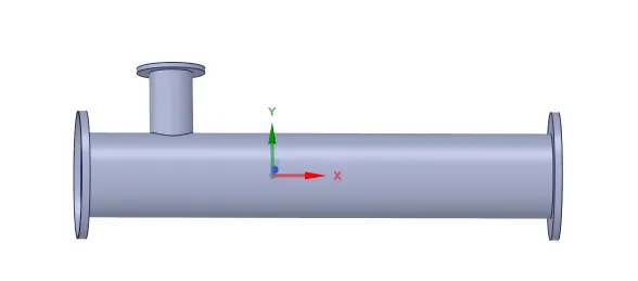
Mixing Tee is shown below in the figure.
Mixing tee possess two inlets and one outlet. The momentum ratio for this type of tee is the ratio of velocity of cold fluid to velocity at mixed fluid at outlet.
Mixing of the fluids inside the pipe was simulated using ANSYS Fluent, a general purpose three dimensional CFD package. The turbulence model selected to setup the required case was k-ℇ. Though Large Eddy Simulations (LES) and Direct Numerical Simulation (DNS) will give most accurate results in this case as it involves turbulent mixing, but many experiments have agreed to the fact that k- ℇ model reasonably agrees with the experimental results. As mentioned above, governing equations i.e. mass and momentum equations are solved using numerical methods as DNS would consume a lot more computational power and time. So we are taking k-ℇ and also we are checking for the `k-omega` also.
K-epsilon.
This model is essentially a high Reynolds number model, meaning the law of the wall must be employed and provide velocity “boundary conditions” away from solid boundaries (what is termed “wall-functions”). Another major drawback is the model's lack of sensitivity to adverse pressure-gradient. It was observed that under such conditions it overestimates the shear stress and by that delays separation.
This model is usually used where flow does not demand to integrate the solution through the viscous sublayer and wall-bounded effects are secondary. For such cases, the first cell away from the wall shall be placed at a y+ of 30-300. In such a scenario, the viscous sublayer and buffer layer (viscosity-affected inner region) are not resolved. Instead, semi-empirical formulas called “wall functions” are used to bridge the viscosity-affected region between the wall and the fully-turbulent region.
K-omega.
K-omega model:
This model is essentially a low Reynolds number model. This model takes 'elliptic' near-wall behaviour meaning that it has an inherent nature of being able to “communicate” with the wall and actually has Dirichlet (as in no-slip in this case) boundary conditions. The implication of such behaviour is the straightforward possibility of integrating through the laminar sublayer without additional numerically destabilizing damping functions or two additional transport equations.
Commonly encountered situations where the flow demands integrating through the viscous sublayer include: heat transfer, calculation of aerodynamic drag, flows with adverse pressure gradients, etc. Integrating through the viscous sublayer would generally impose resolving the mesh to y+<1. The omega equation can be integrated through the viscous sublayer without the need for a two-layer approach
Geometry.
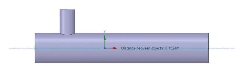
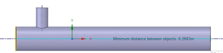
Two geometries of mixing tees were prepared for the analysis in CAD software. One with an outlet length of 0.1924 m
and others with an outlet length of 0.2683 m from T junction which can be observed from Fig. 1 and Fig. 2 with the same inner and outer
the diameter of 0.0039 m for both.
Fig. 1
Fig. 2
The geometry of tee represents solid domain. Fluid domain was required for simulation which was obtained by volume extract feature.
Mesh
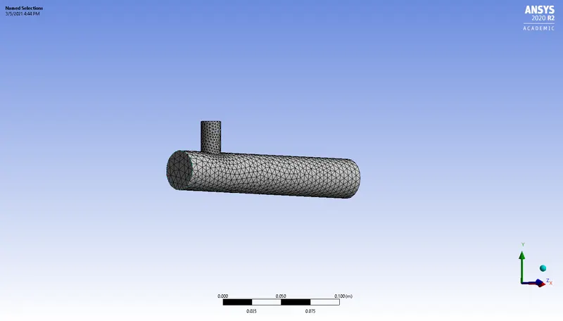
Once the numerically acceptable fluid domain was created, the geometry of tee is imported into ANSYS. The meshing of both tees is
done. Tetrahedral elements with the following cell count were done
for the short tee.
Cell count.
Elements: 12583
Nodes: 2797
Element size: 1.0219e-002m
And for the long tee.
Cell count:
Elements: 15368
Nodes: 3432
Element size: 1.3853e-002m
BOUNDARY CONDITIONS.
Boundary condition is set to inlet-velocity and the outlet is set as the pressure-outlet the velocities of the fluid at both the inlets are entered and the gauge pressure at the outlet will be 0. The fluid here taken is air so the density of the air is 1.2041 kg/m^3 at 19 degree celsius and 1.2754 kg/m^3 at 36 degree celsius. The density and the temperature are taken as cold inlet and the hot inlet fluid respectively.
| parameters |
short tee |
long tee |
| |
K-EPSILON |
K-OMEGA |
K-EPSILON |
K-OMEGA |
| |
CASE 1 |
CASE 2 |
CASE 3 |
CASE 4 |
CASE 5 |
CASE 6 |
CASE 7 |
CASE 8 |
| velocity at inlet-x |
3 m/s |
3 m/s |
3 m/s |
3 m/s |
3 m/s |
3 m/s |
3 m/s |
3 m/s |
| velocity at inlet-y |
6 m/s |
12 m/s |
6 m/s |
12 m/s |
6 m/s |
12 m/s |
6 m/s |
12 m/s |
RESULTS.
CASE 1.
simulation of short tee with the momentum ratio 2. Using the k-epsilon model.
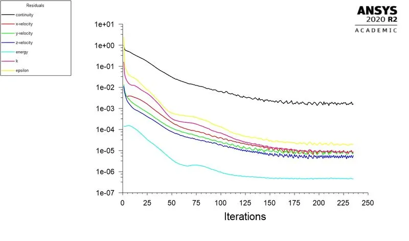
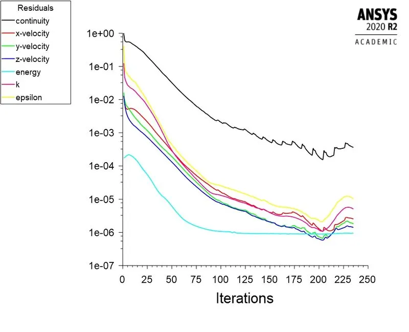
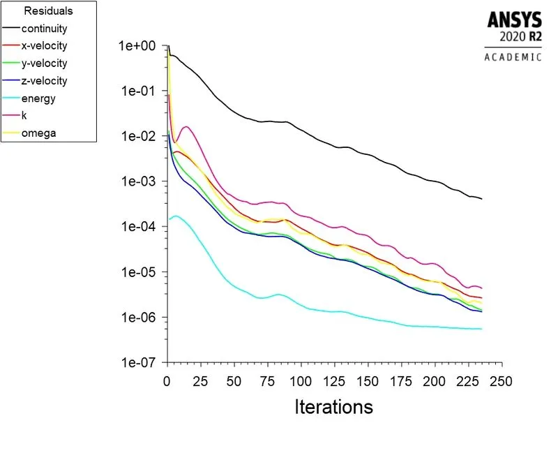
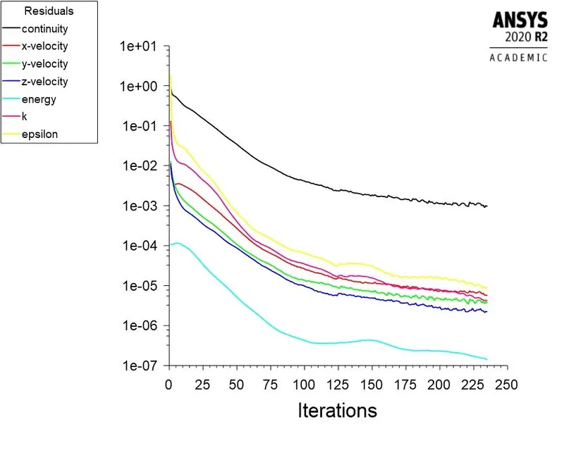
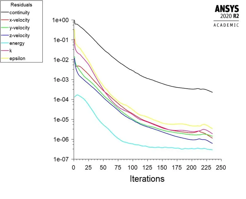
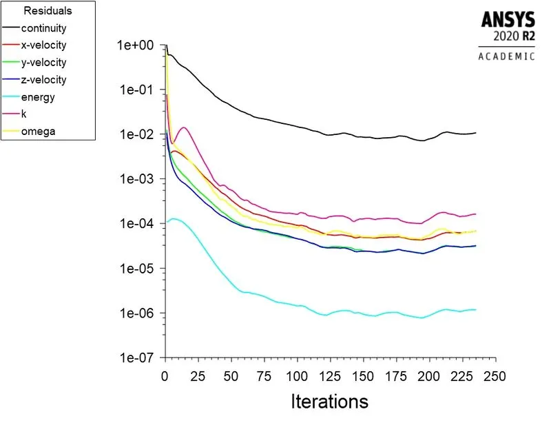
Residuals.
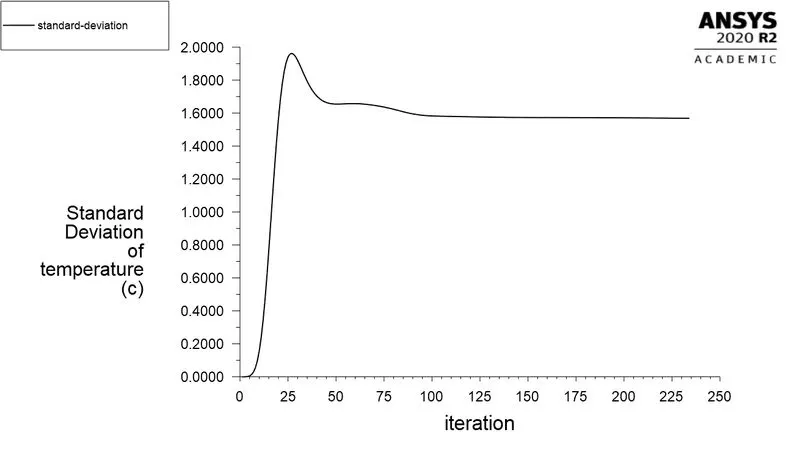
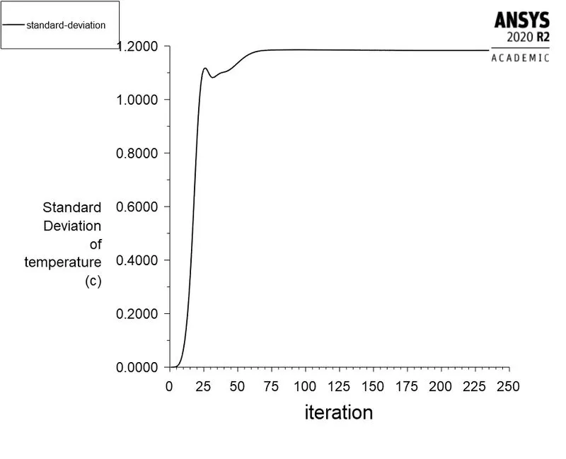
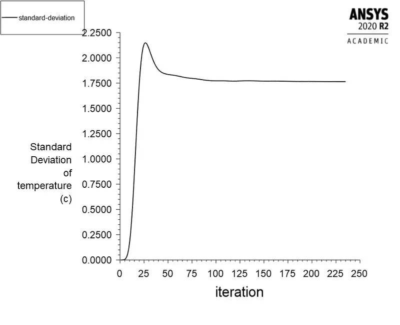
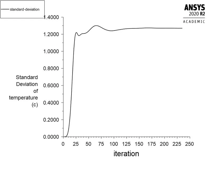
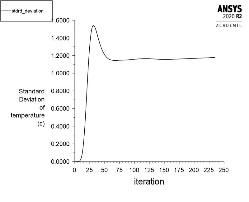
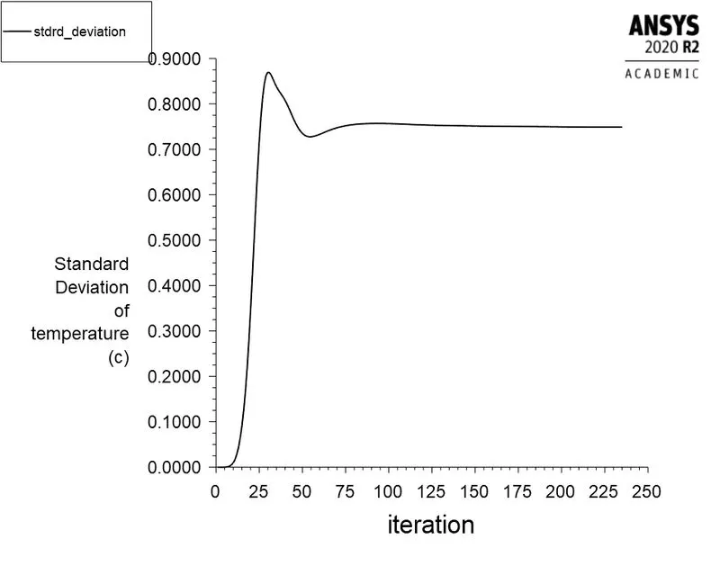
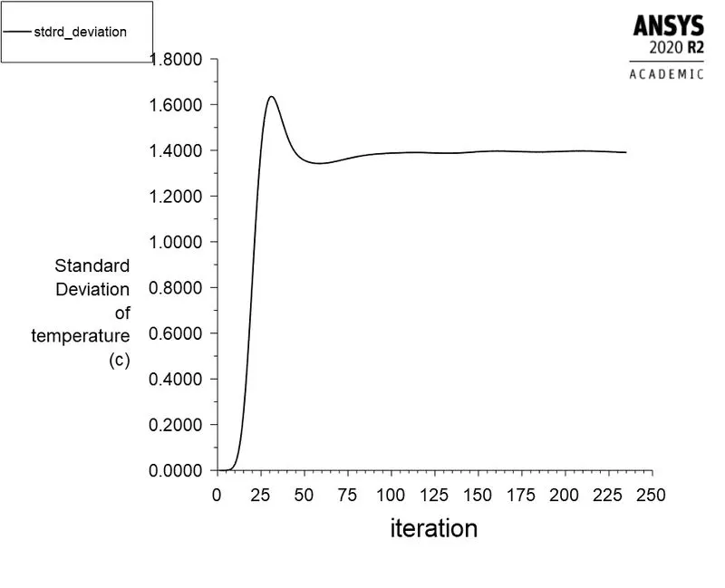
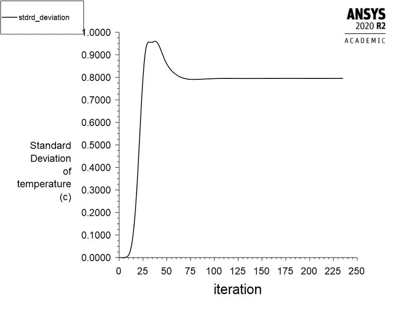
Standard deviation of temperature.
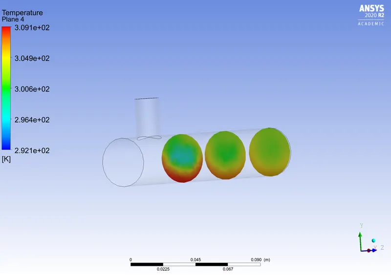
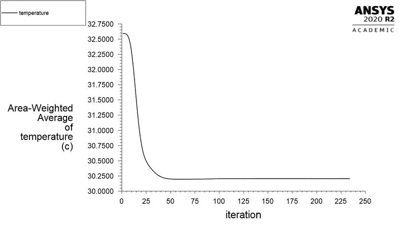
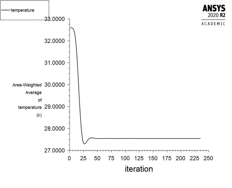
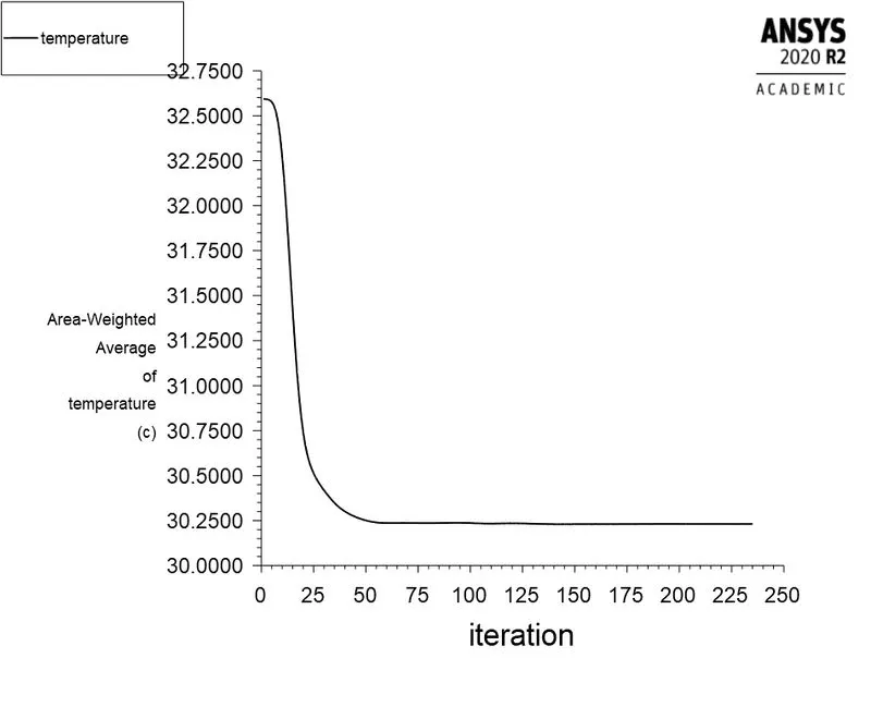
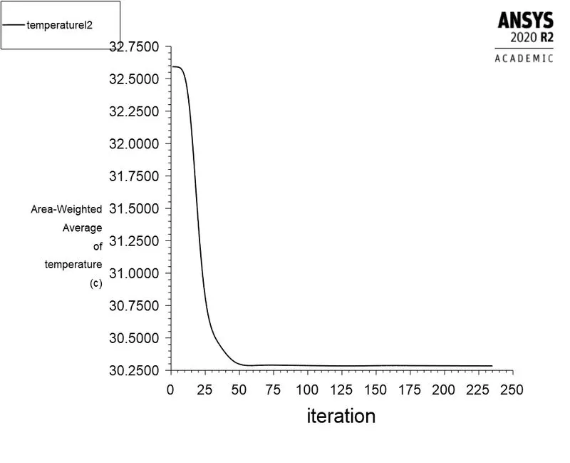
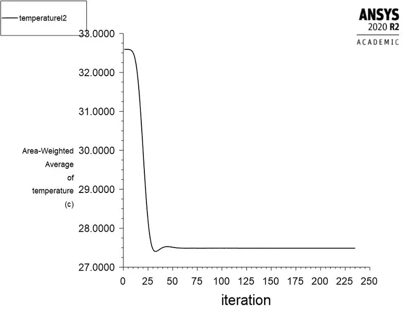
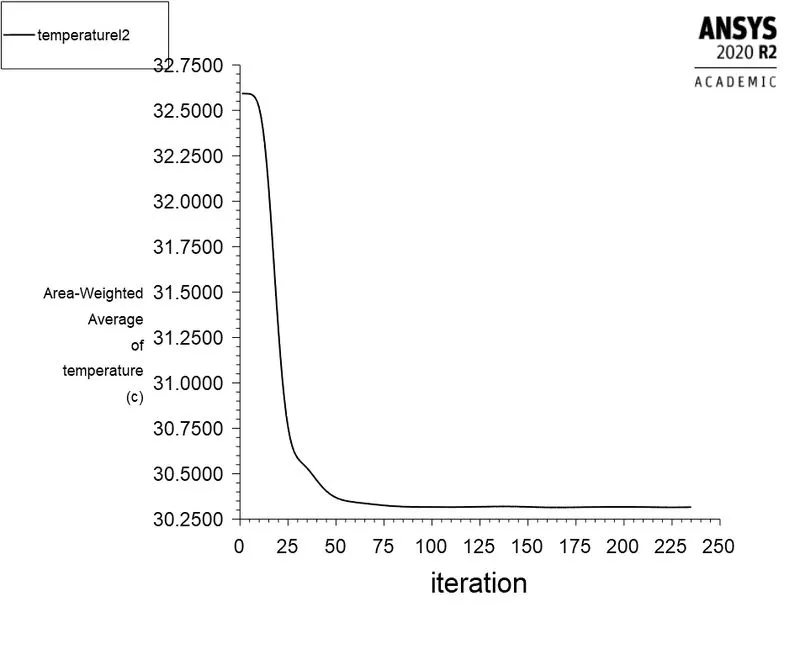
Average temperature at the outlet.
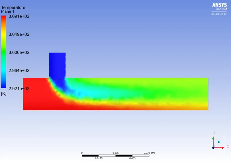
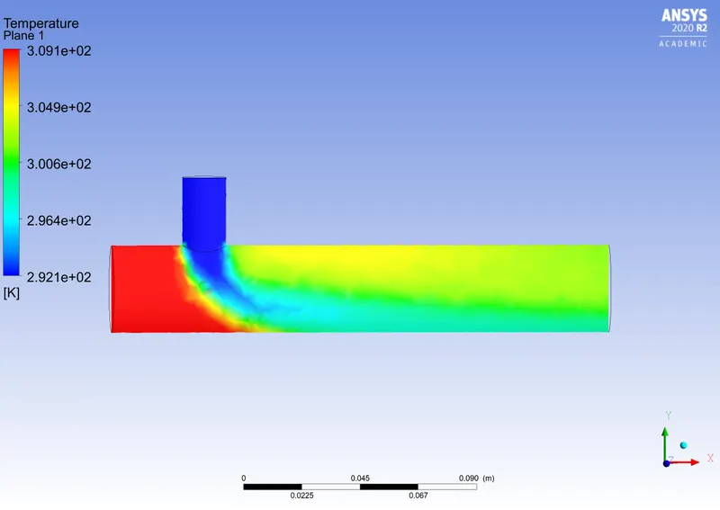
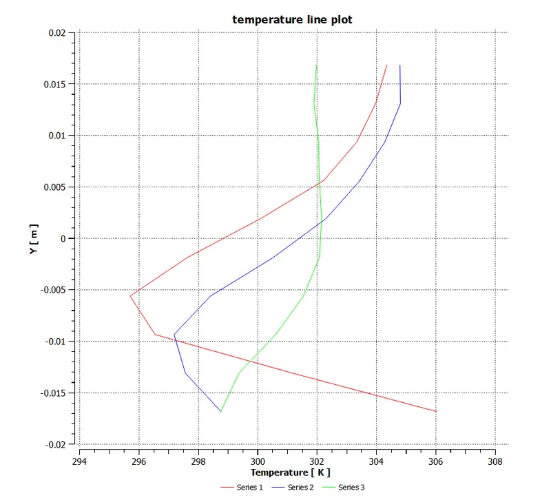
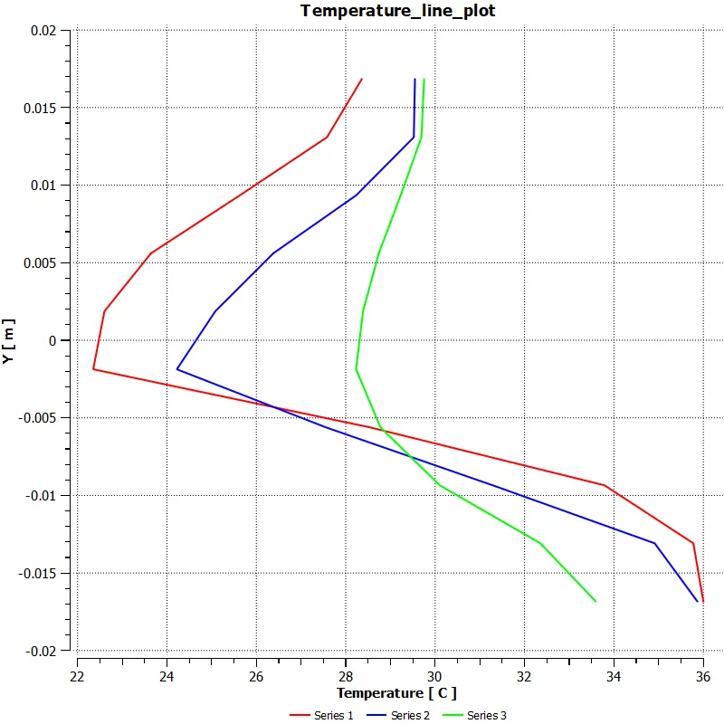
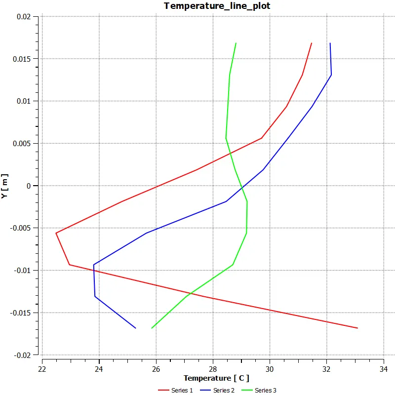
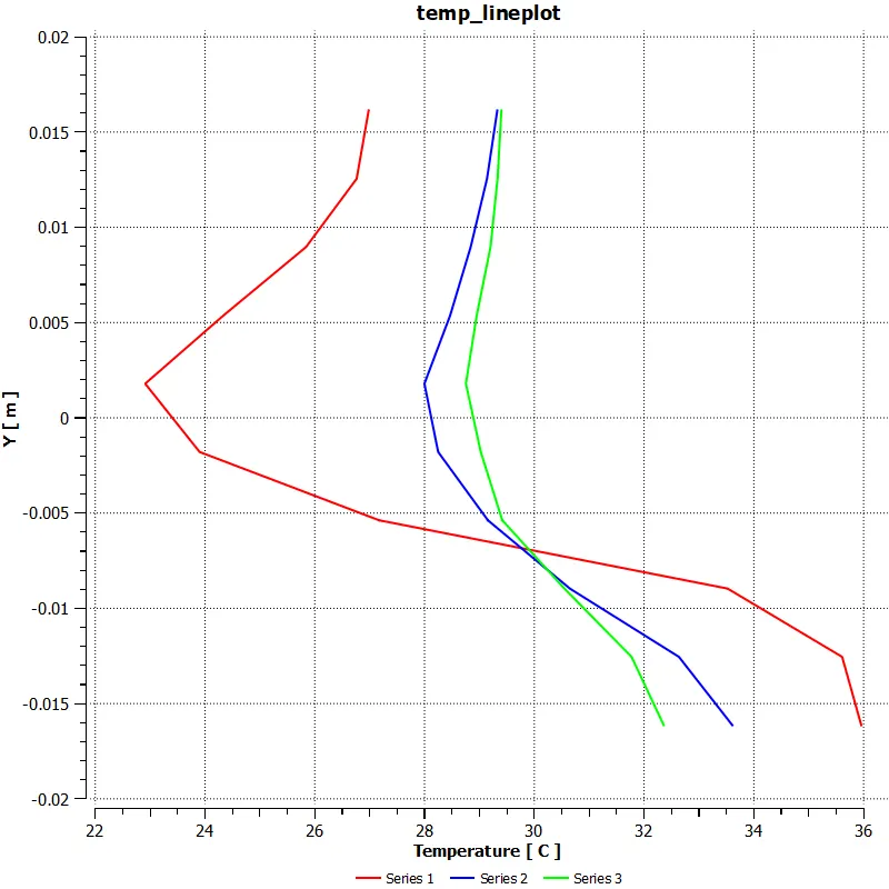
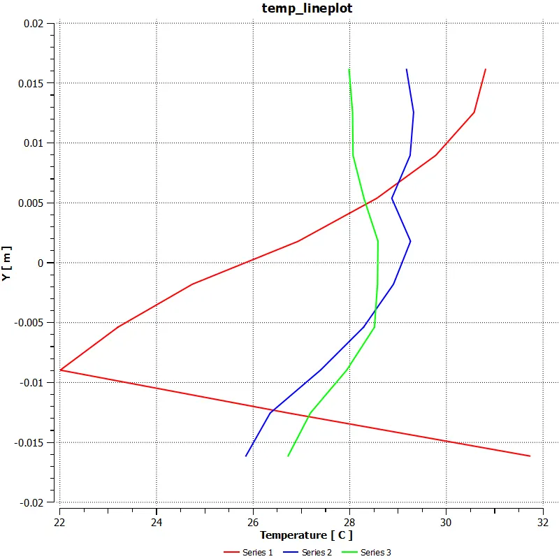
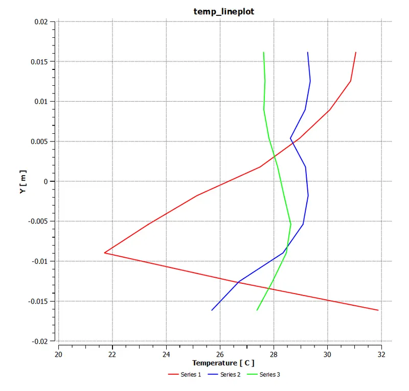
Temperature line plot.
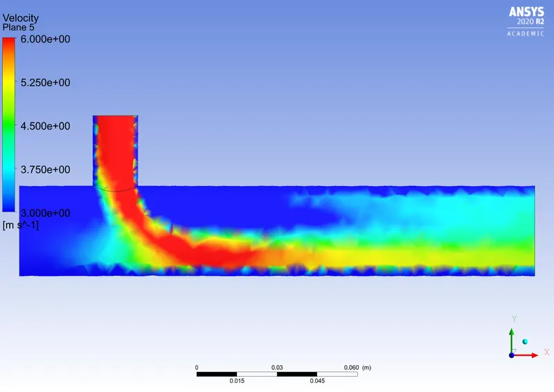
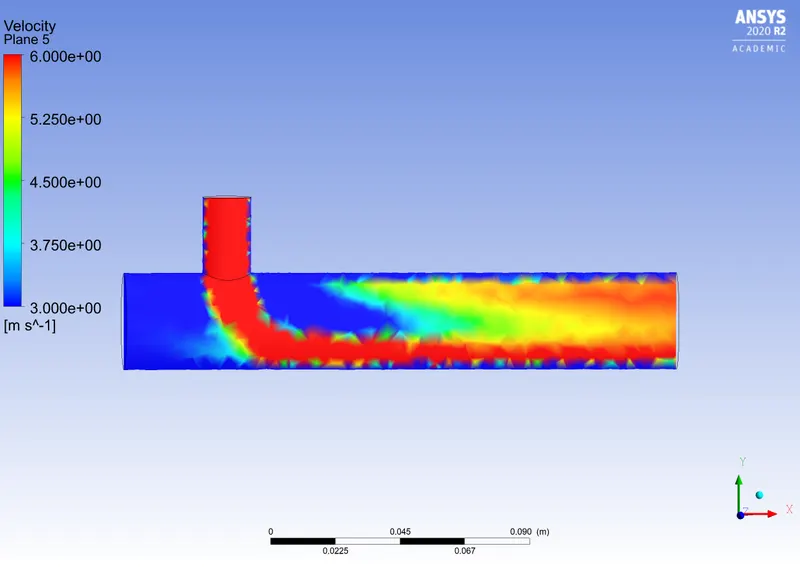
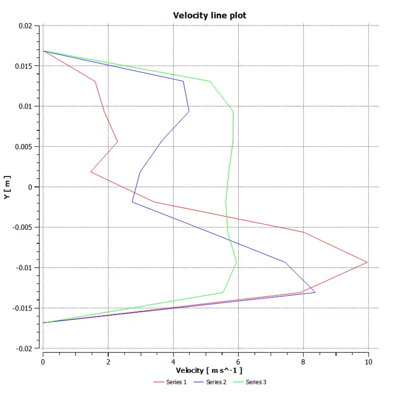
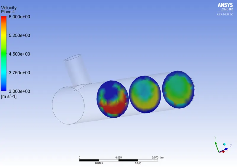
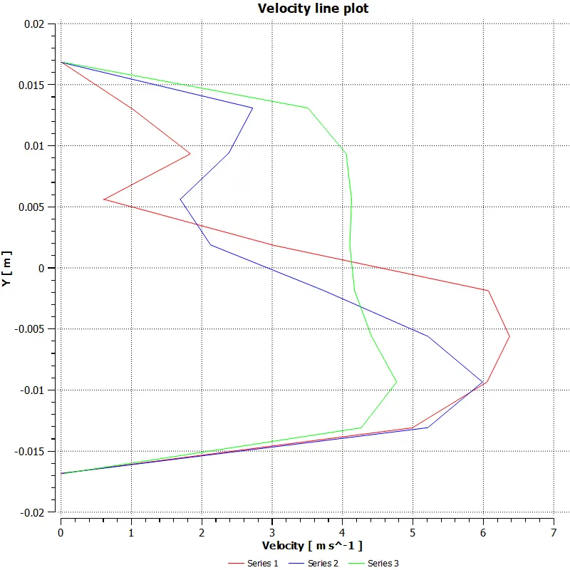
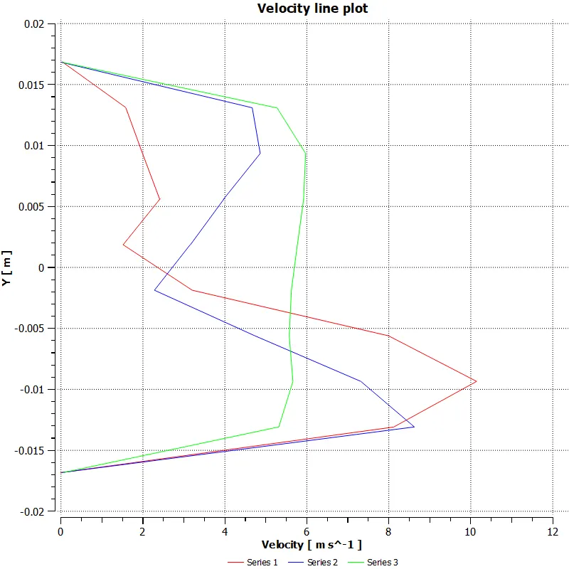
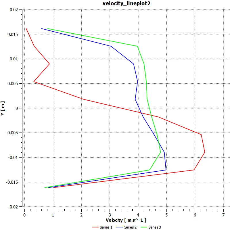
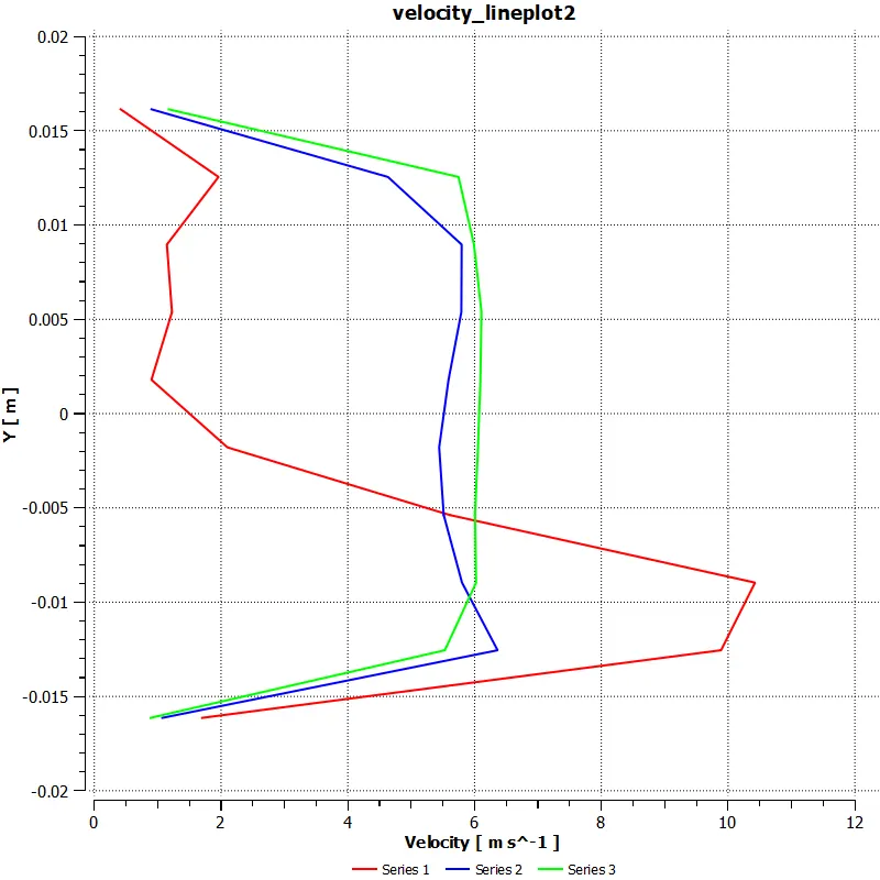
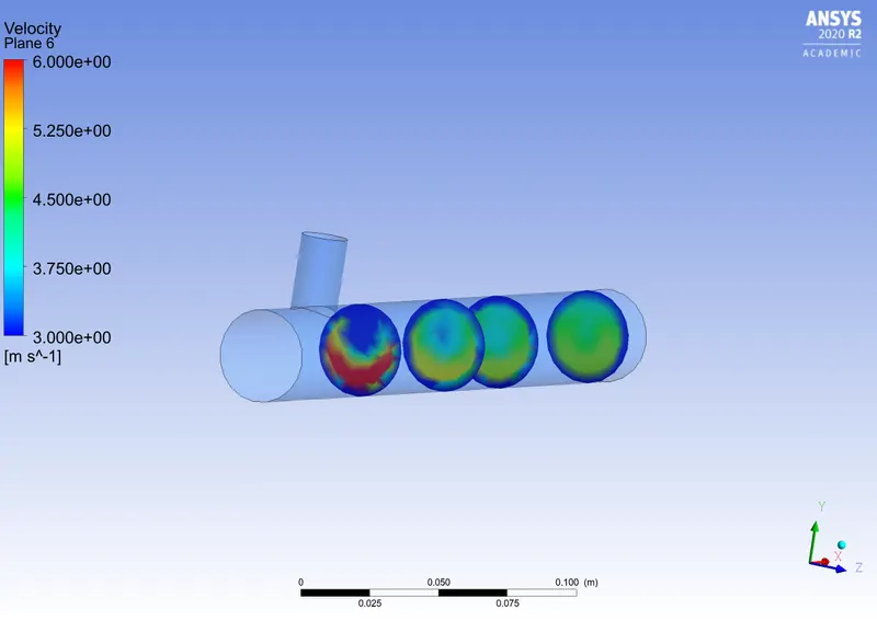
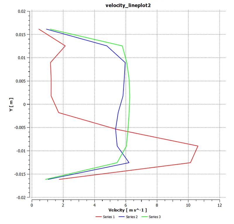
Velocity line plot.
CASE 2.
simulation of short tee with the momentum ratio 4. Using the k-epsilon model.
Residuals.
Average temperature at the outlet.
Standard deviation of the temperature.
Temperature line plot.
Velocity line plot.
CASE 3.
simulation of short tee with the momentum ratio 2. Using the k-omega turbulence model.
Rsiduals.
Average temperature at the outlet.
Standard temperature deviation.
Temperature line plot.
Velocity line plot.
CASE 4.
simulation of short tee with the momentum ratio 4. Using the k-OMEGA model.
Residuals.
Average temperature at the outlet.
Standard deviation of the temperature.
Temperature line plot.
Velocity line plot.
CASE 5.
simulation of long tee with the momentum ratio 2. Using the k-epsilon model.
Residuals.
Average temperature at the outlet.
Standard temperature deviation.
Temperature line plot.
Velocity line plot.
CASE 6.
simulation of short tee with the momentum ratio 4. Using the k-epsilon model.
Residuals.
Average temperature at the outlet.
Standard temperature deviation.
Temperature line plot.
Velocity line plot.
CASE 7.
simulation of short tee with the momentum ratio 2. Using the k-OMEGA model.
Residuals.
Average temperature at the outlet.
Standard temperature deviation.
Temperature line plot.
Velocity line plot.
CASE 8.
simulation of short tee with the momentum ratio 4. Using the k-OMEGA model.
Residuals.
Average temperature at the outlet.
Standard deviation of temperature.
Temperature line plot.
Velocity line plot.
MESH INDEPENDENCE STUDY HAS DONE FOR CASE 1.
THE RESULTS ARE AS FOLLOWS
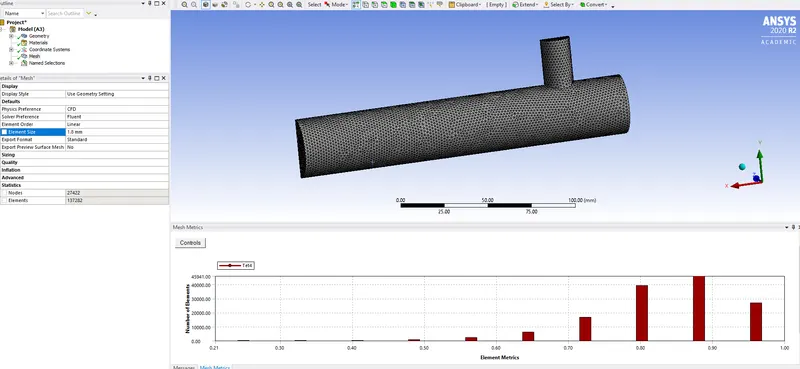
MESH BLOCK.
Cell counts:
Element size: 1.8mm
Nodes: 27422
Elements: 137282
RESULTS.
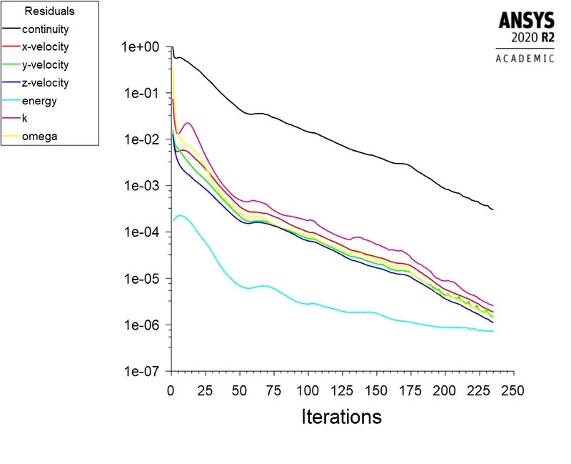
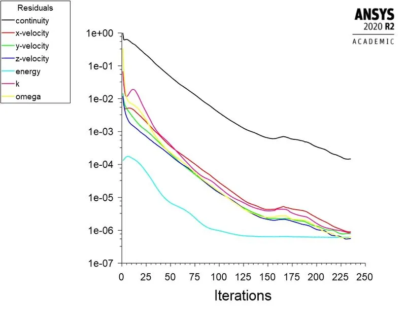
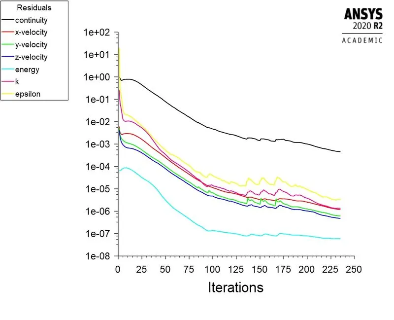
Residuals.
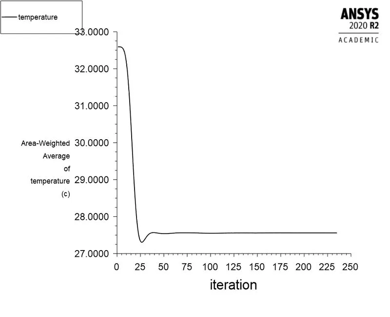
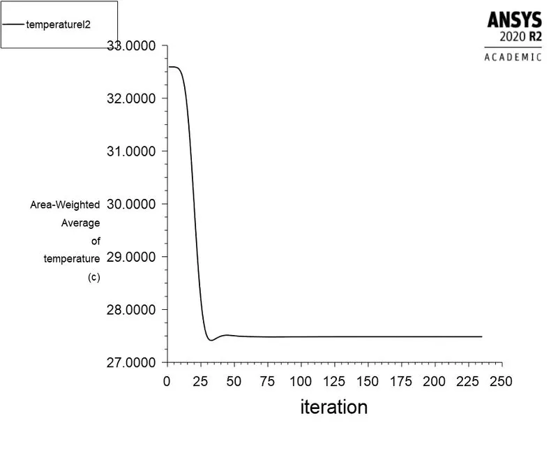
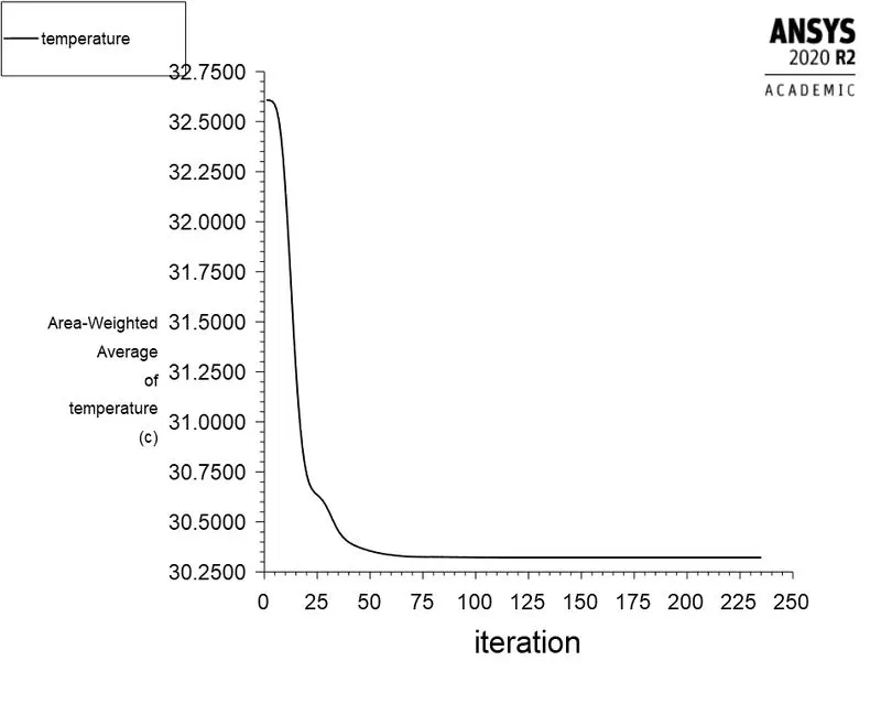
Average temperature at the outlet.
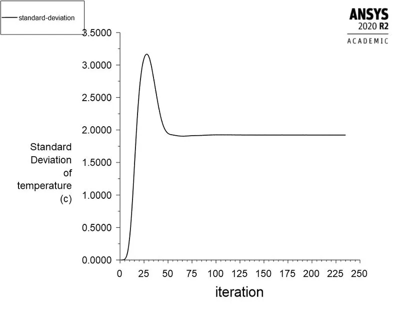
Standard temperature deviation.
MESH INDEPENDENCE STUDY RESULTS
| SHORT TEE |
TURBULENCE MODEL |
MOMENTUM RATIO |
STANDARD DEVIATION OF THE TEMPERATURE |
AREA WEIGHTED AVERAGE TEMPERATURE AT THE OUTLET |
NO. OF ITERATIONS |
| CASE 1 |
k-epsilon |
2 |
1.9225402 |
30.32 |
235 |
| |
|
|
|
|
|
Comparing all the cases that we have simulated.
Here I have taken the same number of iterations for all the cases.
| SHORT TEE |
TURBULENCE MODEL |
MOMENTUM RATIO |
STANDARD DEVIATION OF THE TEMPERATURE |
AREA WEIGHTED AVERAGE TEMPERATURE AT THE OUTLET |
NO. OF ITERATIONS |
| CASE 1 |
k-epsilon |
2 |
1.568100 |
30.2064 |
235 |
| CASE 2 |
k-epsilon |
4 |
1.1833259 |
27.5430 |
235 |
| CASE 3 |
k-omega |
2 |
1.7639253 |
30.2310 |
235 |
| CASE 4 |
k-omega |
4 |
1.2698685 |
27.5587 |
235 |
| |
|
|
|
|
|
| LONG TEE |
|
|
|
|
|
| CASE 1 |
k-epsilon |
2 |
1.1779499 |
30.2801 |
235 |
| CASE 2 |
k-epsilon |
4 |
0.7487151 |
27.4877 |
235 |
| CASE 3 |
k-omega |
2 |
1.3902929 |
30.3159 |
235 |
| CASE 4 |
k-omega |
4 |
0.7951669 |
27.4865 |
235 |
CONCLUSION.
From the result of the area weighted-average of temperature at the outlet, it can be observed that the temperature at the outlet shows no significant change when the velocity is the same even though the length of the outlet is increased from the junction. But it has been observed that the outlet temperature shows a significant decrease when the momentum ratio is increased resulting in increased mixing efficiency.
The above-mentioned behaviour is also the same for the results of the standard deviation of temperature at the outlet. Hence, on the basis of
obtained results and observations made, case 2 in both the long and short tees yields more mixing efficiency relative to other cases. Hence mixing tee efficiency momentum ratio. Also, the increase in the length of tee does not play any significant role as compared to the increase in momentum ratio on the efficiency of Mixing tee.