Week 1- Mixing Tee

Aim:

To simulate a flow through mixing tee and understand the mixing effectiveness based on length of the mixing tee and the momentum ratio given that the hot inlet temperature is `36^0`C and the cold inlet is at `19^0`C.

Theory:

Mixing Tees utilizes a specifically engineered internal geometry to efficiently mix two fluid streams into one combined stream. Mixing tees are widely used in the petrochemical, HVAC industry etc.

In given problem, we have the hot air at `36^o`C and cold air at `19^o`C. As per CAD, the velocity inlet in x-direction is for hot air and the velocity inlet in y-direction is for cold air.

We have given two cases viz.

Case 1

• Short mixing tee with a hot inlet velocity of 3m/s
• Momentum ratio of 2, 4

Case 2

• Long mixing tee with a hot inlet velocity of 3m/s
• Momentum ratio of 2, 4

Objectives:

• To compare the cell count, average outlet temperature, number of iterations for convergence from 2 cases
• To plot velocity and temperature contours/line for given cases
• To perform mesh independent study for any one case
• To discuss the effect of length and momentum ratio on results

Steps followed for simulation:

Pre-processing

This step includes geometry cleanup and volume extraction for further preocessing. After extracting the volume, fluid zone is discretised into cells which is called meshing. After meshing, boundaries are defined.

In case setup, the boundaries defined earlier are given specific conditions like inlet, oulet, walls with values. Energy model is turned on and suitable turbulence model is selected.

Solving

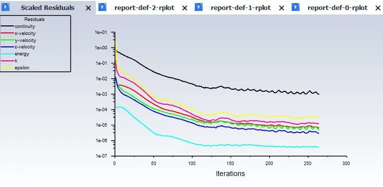
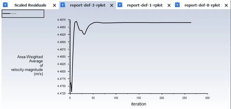
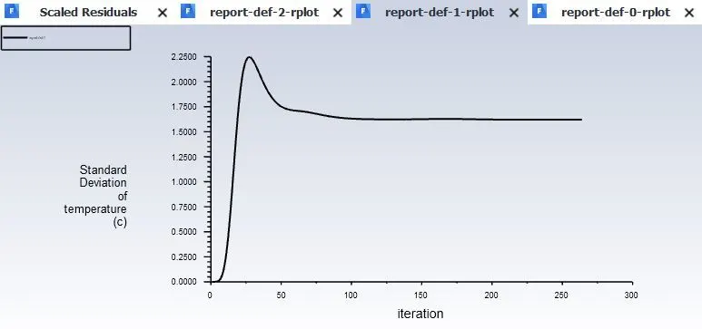
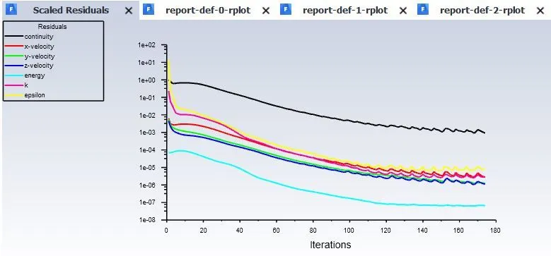
Number of iterations are set to achieve convergence. While solving, some monitors are set i.e. standard deviation, area weighted average of velocity and temperature at outlet. This gives us the idea about how the run is proceeding.

Post-processing

Velocity and temperature contours are plotted on the cut planes along and across the pipe. The effect of length and momentum ratio was observed. Also, the effect of turbulence model was observed.

Baseline simulation:

For hot inlet velocity of 3 m/s and momentum ratio 2

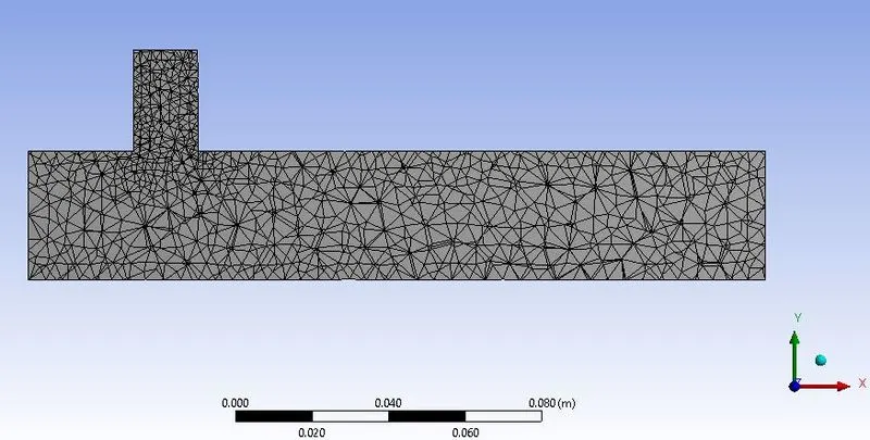
Default mesh size - 1.0219e-002 m

Mesh

Number of elements - 12,760

Residuals

Standard deviation

Velocity:

Temperature:

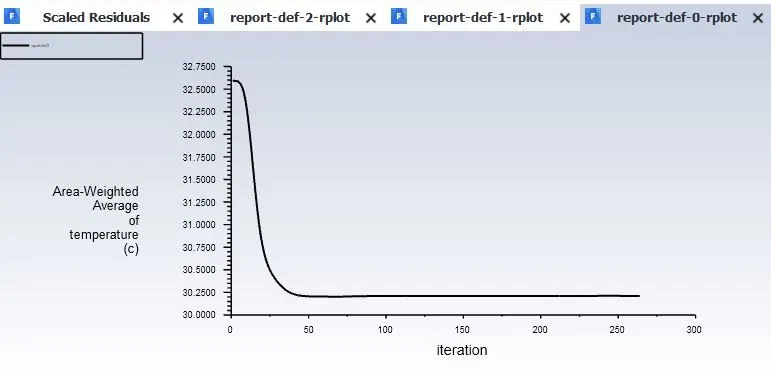
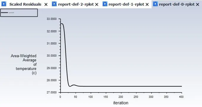
Area-Weighted average

Temperature:

Contours

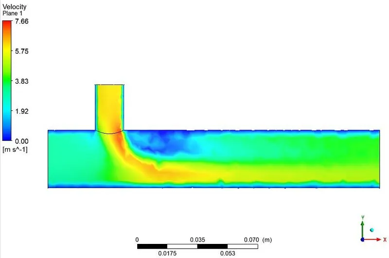
Velocity:

Temperature:

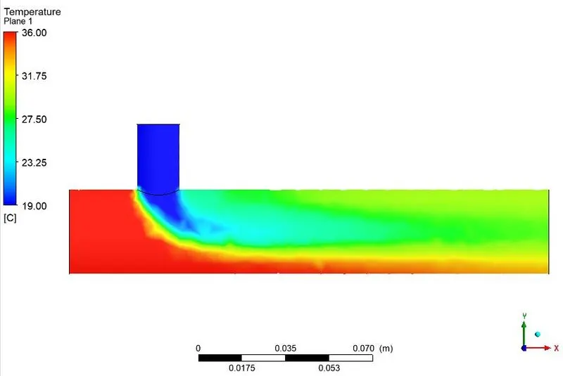
In this baseline simulation, the mesh is coarse. As a result, the temperature and velocity contours are diffused. So, it is required to go for finer mesh.

Case 1 - Short mixing tee

a) For hot inlet velocity of 3 m/s and momentum ratio 2

Mesh size - 2e-03 m

Number of elements - 105746

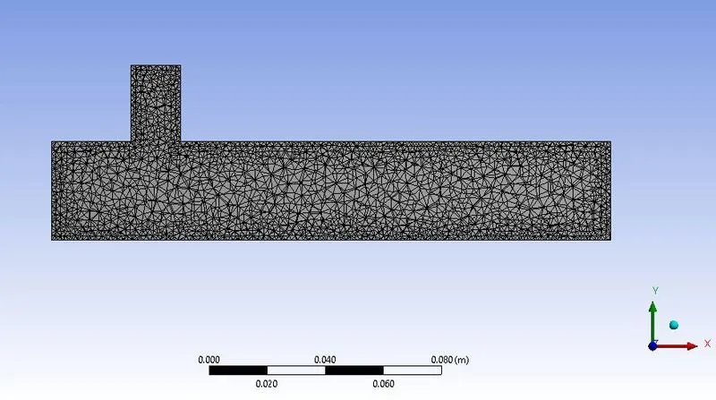
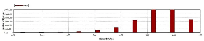
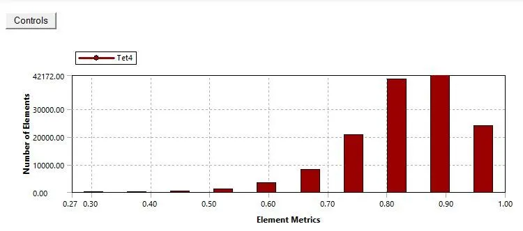
AAs compare to previous meshed model, this has more high quality elements ranging between 0.8 to 0.9. So, this mesh is acceptable.

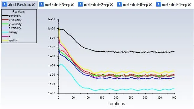
Residuals

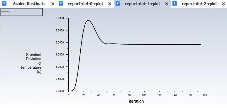
Standard deviation

Temperature:

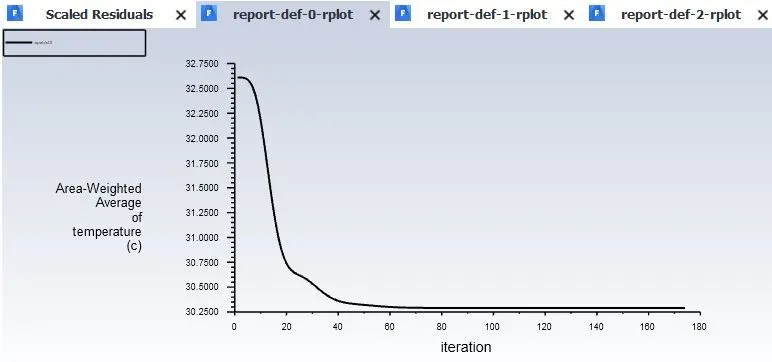
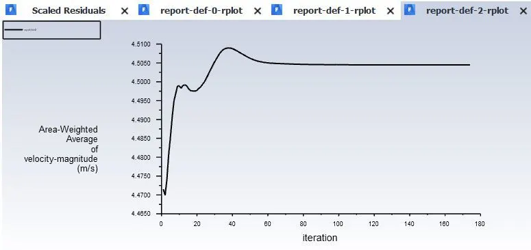
Area-weighted average

Temperature:

Velocity:

Contours

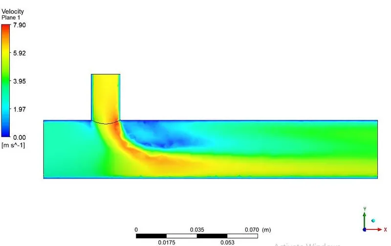
Velocity:

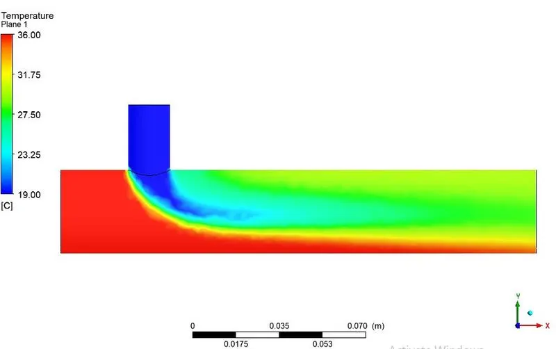
Temperature:

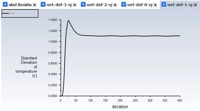
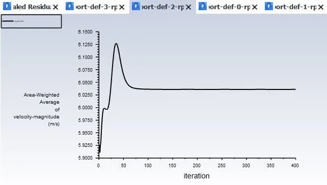
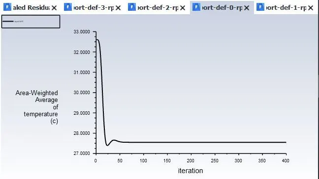
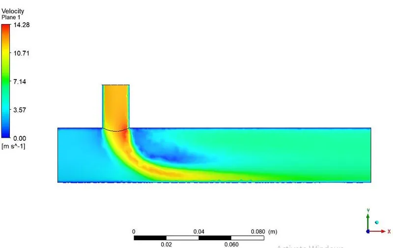
b) For hot inlet velocity of 3 m/s and momentum ratio 4

Meshed model remains same as previous i.e. mesh size 2e-03 m.

Residuals

Standard deviation

Temperature:

Area-weighted average

Velocity:

Temperature:

Contours

Velocity:

Temperature:

Case 2 - Long mixing tee

a) For hot inlet velocity of 3 m/s and momentum ratio 2

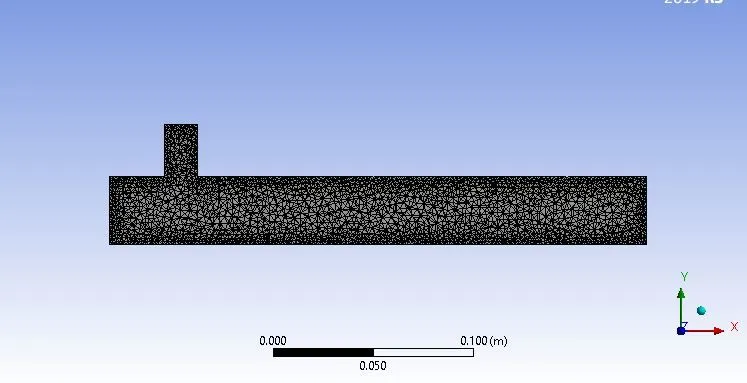
Mesh size - 2e-03 m

Number of elements -

The mesh size is kept same as previous case.

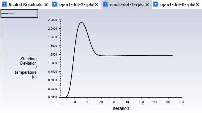
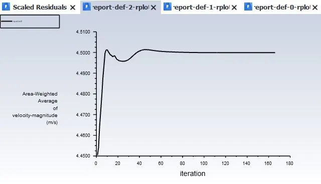
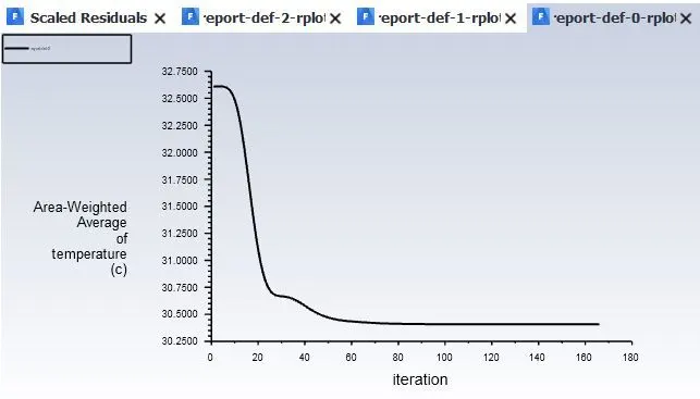
Residuals

Standard deviation

Temperature:

Area-weighted average

Velocity:

Temperature:

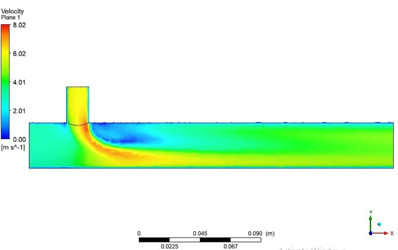
Contours

Velocity:

Temperature:

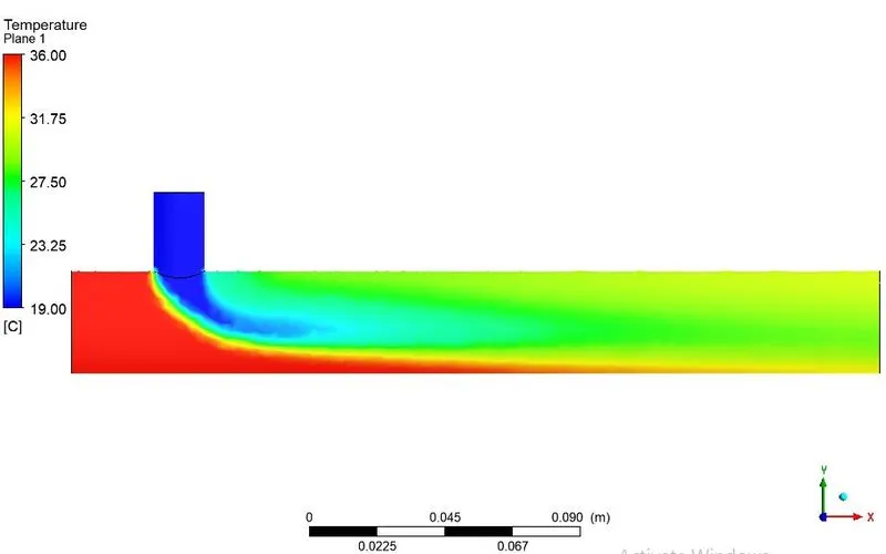
b) For hot inlet velocity of 3 m/s and momentum ratio 4

Mesh size - 2e-03 m

Number of elements -

The mesh size is kept same as previous case.

Residuals

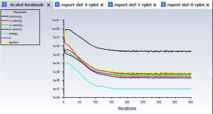
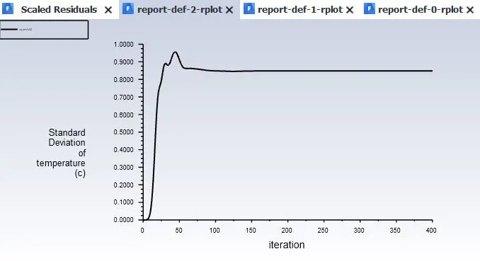
Standard deviation

Temperature:

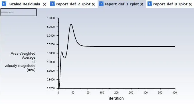
Area-weighted average

Velocity:

Temperature:

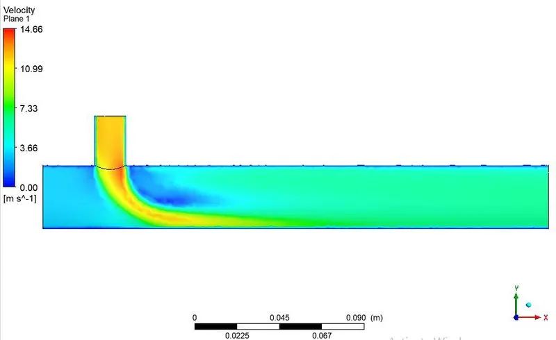
Contours

Velocity:

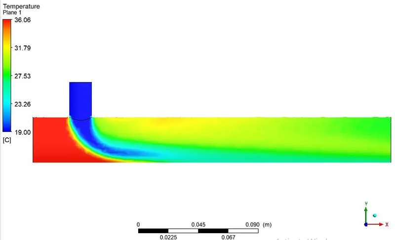
Temperature:

Effect of Turbulence model

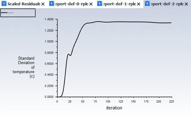
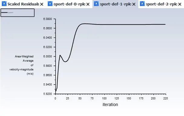
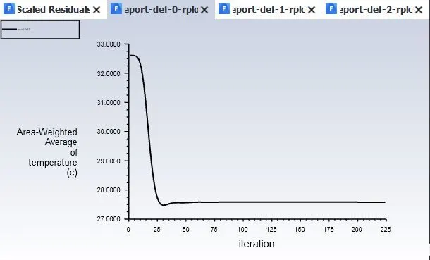
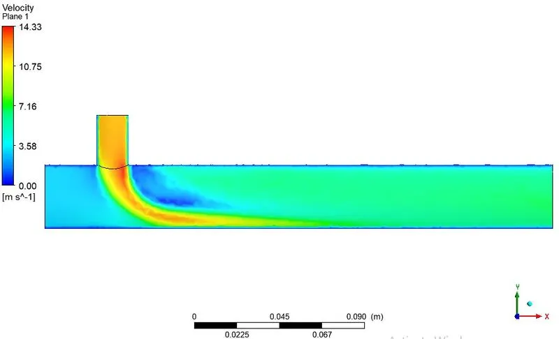
SST k-`omega` model is used for the previous case i.e. Case 2 - Long mixing tee for hot inlet velocity of 3 m/s and momentum ratio 4. Mesh parameters remains same as previous.

Residuals

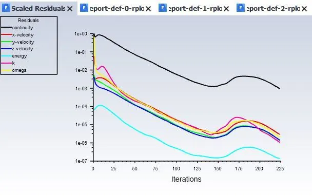
Standard deviation

Temperature:

Area-weighted average

Velocity:

Temperature:

Contours

Velocity:

Temperature:

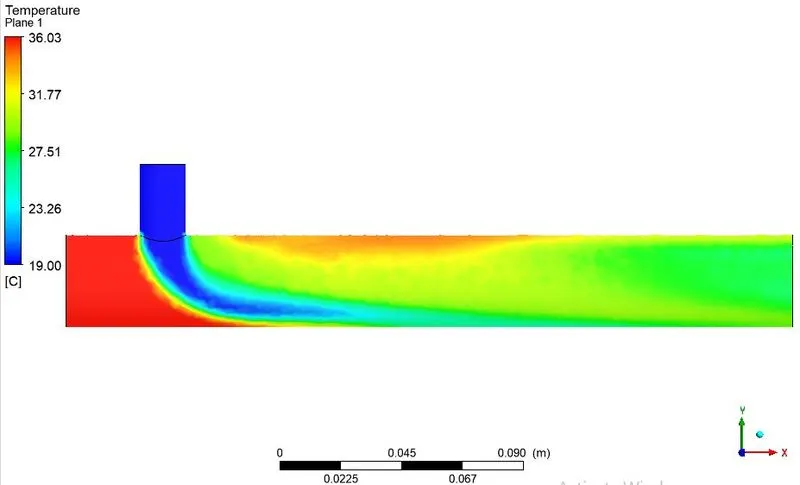
Comparison among given cases

Case	Element count	Average outlet temperature (Deg C)	Number of iteartions for convergence
Short tee - M.R. 2	105746	30.3	170
Short tee - M.R. 4	105746	27.5	200
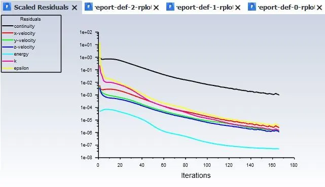
Long tee - M.R. 2	140042	30.4	170
Long tee - M.R. 4	140042	27.5	200

Conclusion

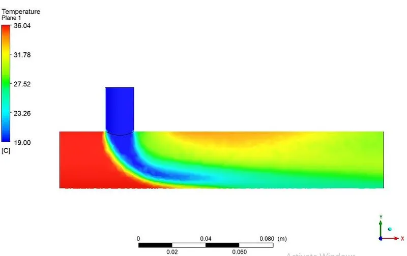
1. When we compare Case 1-a with Case 1-b, one can observe the change in temperature drop. In prior case, due to lower velocity of cold air, there is no effective mixing. So, the average temperature at outlet is higher than that of Case 1-b.
2. When we compare Case 1 with Case 2, one can observe in Case 1 that the hot air sips through the oulet without proper mixing with cold air. This is due to insufficient length of mixing. So, to have proper mixing, length of the mixing tee should be sufficiently long.
3. So to have proper mixing, the length of mixing tee and the momentum ratio should be sufficiently high.
4. If we compare the cases with different turbulence models, one can observe that the k- epsilon captures well far from boundary layer. On other hand, k- omega captures well near to the wall (See temperature contours for Case 2 with k- epsilon and k- omega turbulence model).
5. k- epsilon is more accurate when fully turbulent flow is there. Also, it is computationally cheap with respect to the k- omega. Here, we are interested to see the mixing effectiveness not near wall tempeartures. So, for this k- epsilon is better that k-omega.