Mixing Tee

OBJECTIVE

To set up steady-state simulations at a Tee-Joint to compare the mixing effectiveness when hot inlet temperature is 36⁰C & the Cold inlet is at 19⁰C.

The k-epsilon and k-omega SST models should be used for the first case and based on the judgment use the more suitable model for further cases.

1. Case 1
• Short mixing tee with a hot inlet velocity of 3m/s.
• Momentum ratio of 2 and 4.
2. Case 2
• Long mixing tee with a hot inlet velocity of 3m/s.
• Momentum ratio of 2 and 4.

PROCEDURE/WORKFLOW

• GEOMETRY:
• Let's start with analysing which model (whether K-epsilon or k-omega) is suitable for conducting the simulation. For that, we employ the short mixing tee model, and is imported to spaceclaim geometry.

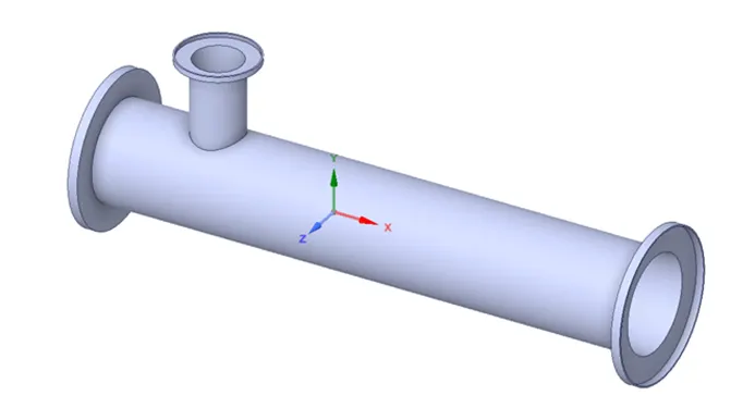
Figure 1: Basic geometry of a short mixing tee joint

The required solid volume is selected and the rest is supressed for physics.

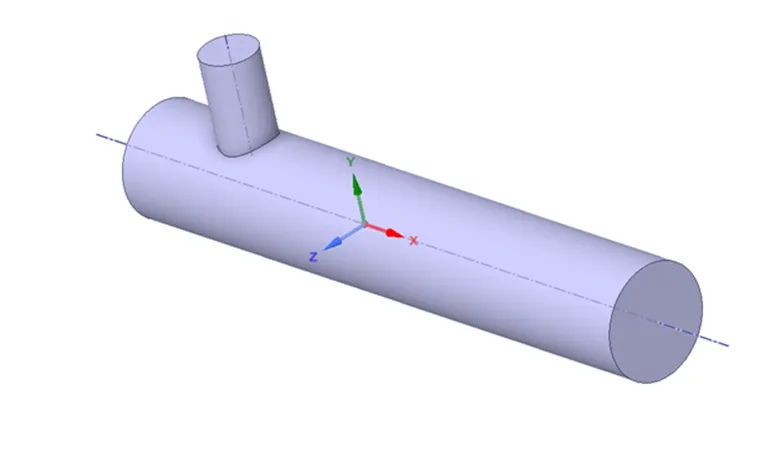
Figure 2: Geometry of a short mixing tee joint after suppressing

• MESH:
• Once the geometry is completed, the meshing process starts. Within the meshing, initially, create the named selections by providing appropriate names and generate the basic mesh.

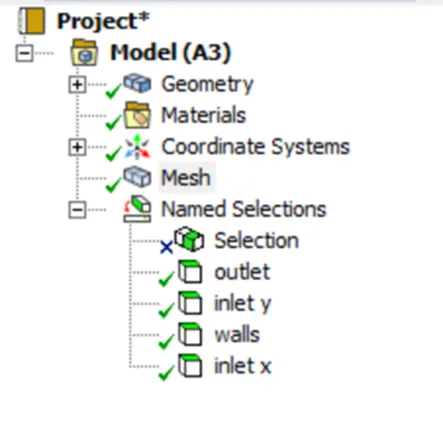
Figure 3: Mesh tab with details of mesh and named selection

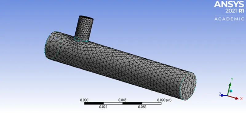
Figure 4: Meshed tee joint

A section plane isa created to evaluate the cross-sectional view of meshing.

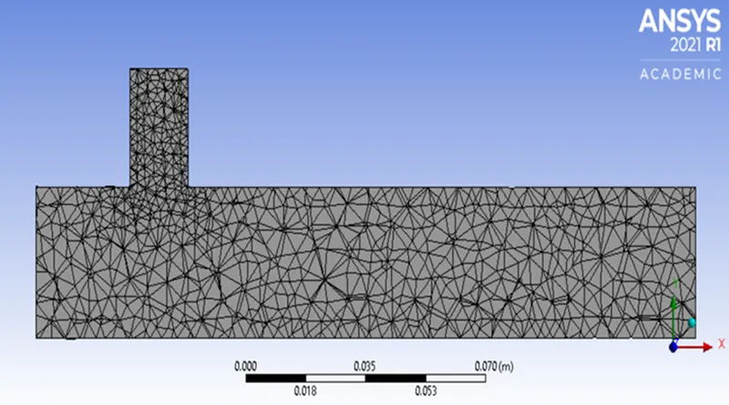
Figure 5: Meshing across the cross-section of the joint

We also investigate the quality of mesh by using element quality option in mesh metrics. The quality of mesh is graded on a scale of 0 to 1, and in our graph, most of our cells fall almost near to 1 and hence can be assumed to be of good quality.

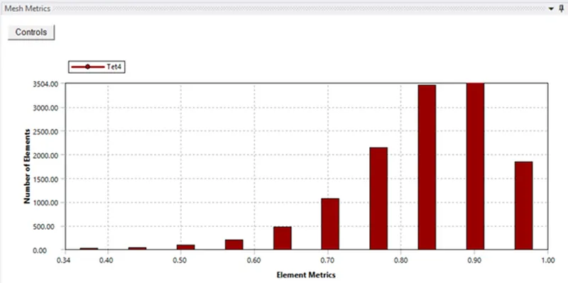
Figure 6: Element quality histogram

• SETUP:
• The setup is launched. If everything works fine, the window will be launched without throwing any error.

The following solvers are selected in the task page.

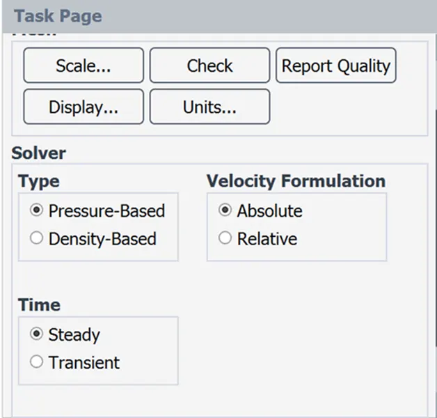
Figure 7: Solver selection conditions

Since we are analysing the k-epsilon model, the following options of realizable and standard wall functions are checked

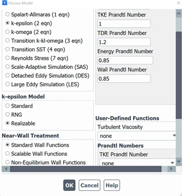
Figure 8: Parameters for K-epsilon model

• In the materials section, make sure that the fluid is air.
• 

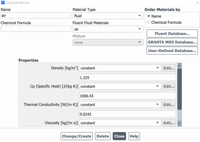
Figure 9: Material selection/editing tab

• The boundary conditions are specified within the boundary in the zones section. For inlet x, the initial velocity is 3m/s and temperature is 36 C whereas for inlet y is 6 m/s (since momentum ratio is 2) and the temperature is 19C. For the outlet, the gauge pressure is kept 0. Later, the momentum ratio is changed to 4.
• 

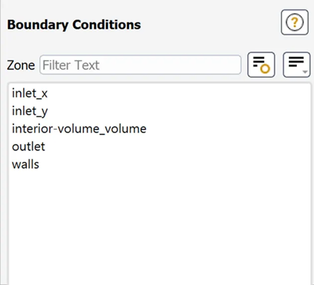
Figure 10: Boundary conditions selection/editing tab

• Inorder to monitor the physical quantities during solving, surface reports of temperature and standard deviation of temperature at outlet are created.

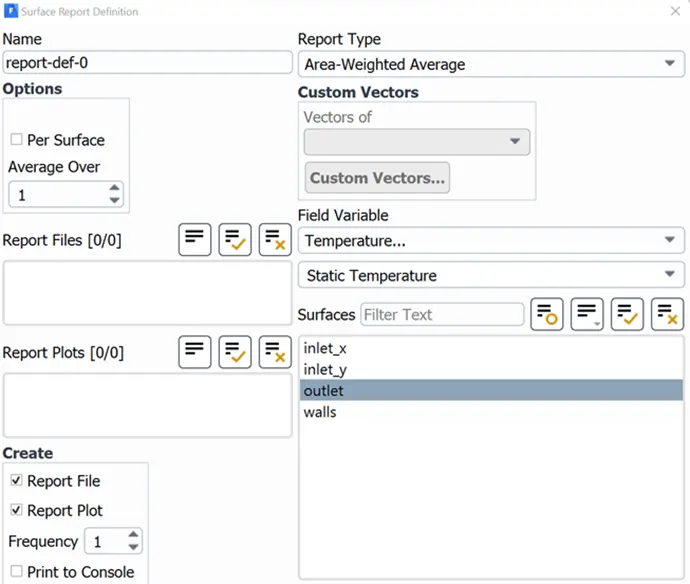
Figure 11: Generation of surface reports

• Initialization: Hybrid initialization is set up and is initialized.

Figure 12: Initialization

After 20 iterations, hybrid initialization is completed.

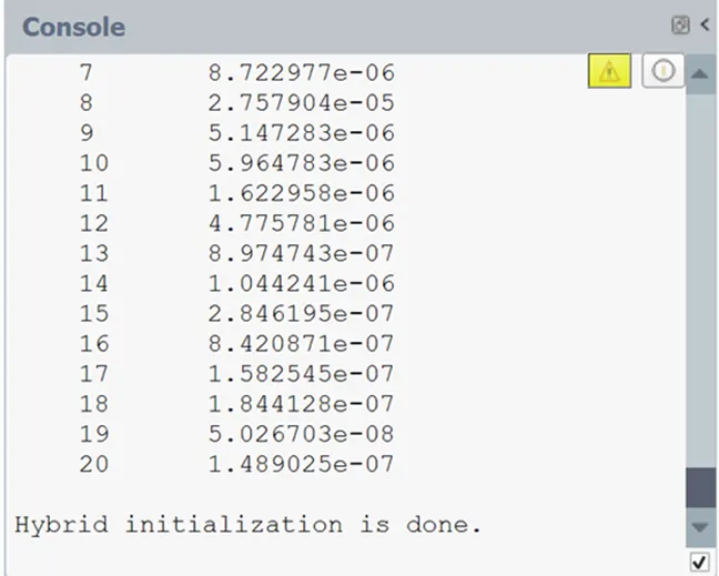
Figure 13: Console window showing the completion of initialization

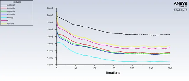
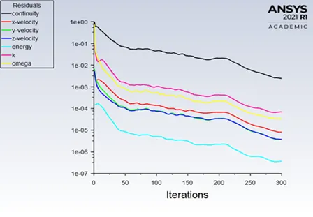
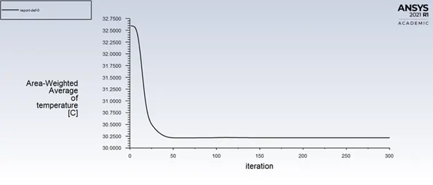
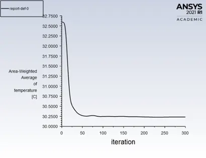
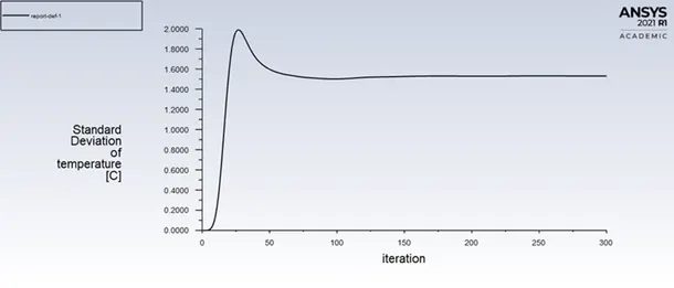
• The calculation is run for 300 iterations and is evaluated whether it gets converged or not. The same procedure is followed for k-omega model as wel, except, we select the k-omega SST model and the mesh convergence is evaluated.

K-epsilon	K-omega

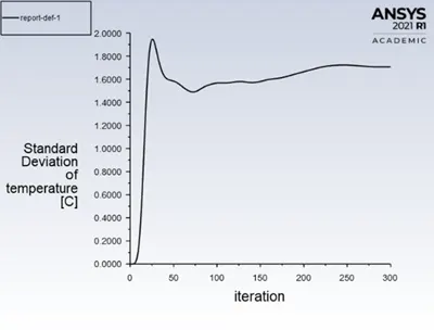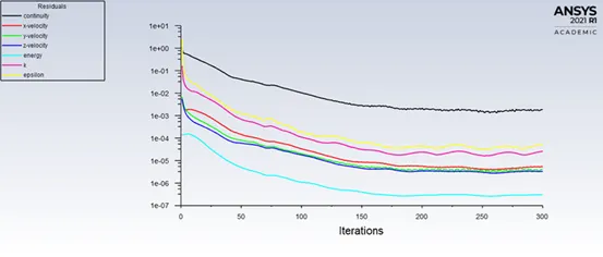
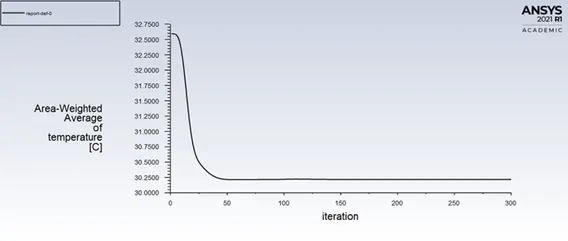
Figure 14: Comparison of residuals, area weighted average of temperature, standard deviation of temperature at outlet for K-epsilon and K-omega model

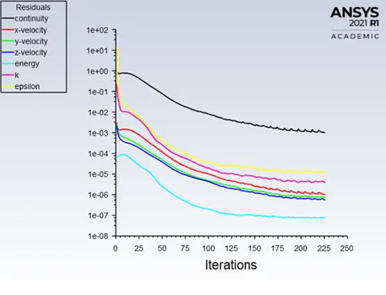
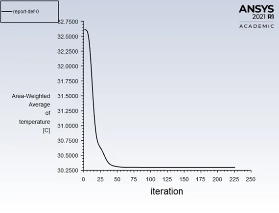
It can be seen from the results that, for the k-epsilon model, we get a converged residual results after about 160 iterations, however, for the k-omega model, the residuals are still converging, even after 300 iterations. Through the generated images, we can see that K-omega model flow is more laminar and is not giving proper turbulent results, in contrast, simulation by K-esilon is giving proper mixing of the two air streams. K-omega model is well suited for viscous sub-layers,i.e, near the wall flow region, whereas K-epsilon model is ideal for predicting flow in regions away from the walls.

Based on this observation, the K-epsilon model is chosen for the simulation process.

MESH/GRID INDEPENDENCE STUDY

The mesh independence study is conducted to analyze the effect of grid size on the results and to select the convenient mesh size for the simulation process.

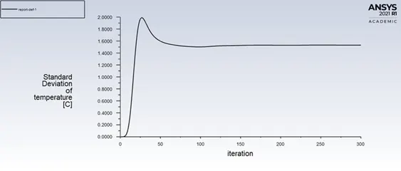
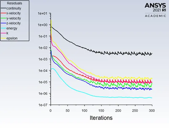
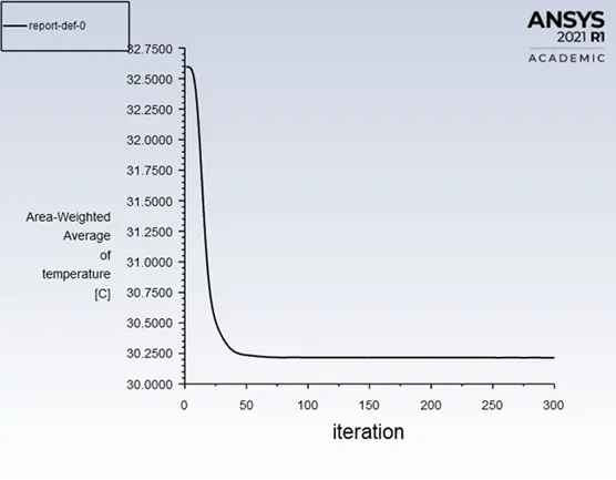
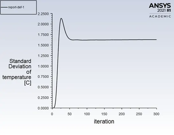
Here, the study is performed on short tee model, with a momentum ratio of 2, taking element sizes as 1.902e-2 (default), 5e-3 and 2e-3. The results are shown below.

1.9e-2
5e-3
2e-3

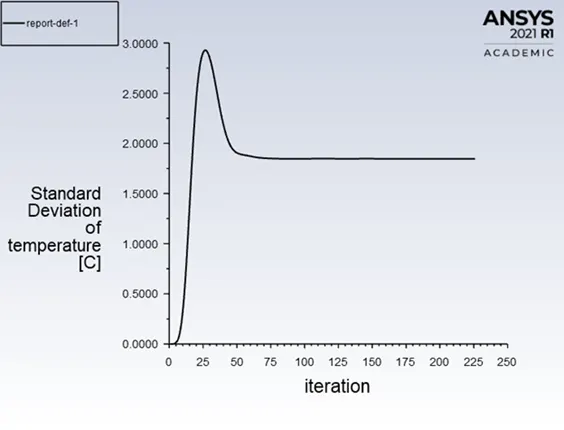Figure 15: Grid independence study for various element sizes

Mesh size(m)	Cell count	Iterations to get converge	Average temperature at outlet (C)	Average velocity at outlet (m/s)
1.902e-2	12728	160	30.25	4.17
5e-3	14228	175	30.25	4.11
2e-3	105168	200	30.30	4.03

Table 1: Results of Grid independence study

It can be seen that, even though the mesh size is getting refined, the average temperature and velocity at the outlet remains unchanged. However, the process takes much more time to converge as more and more equations need to be solved as the grid points are increased. So, either the default or 5e-3 mesh size could be opted. Here, in my study, I have chosen 5e-3.

RESULTS

Case 1 : Mixing Tee Short

a:

Momentum ratio	2
Inlet x velocity	3 m/s
Inlet y velocity	6 m/s
Inlet x temperature	36 C
Inlet y temperature	19 C

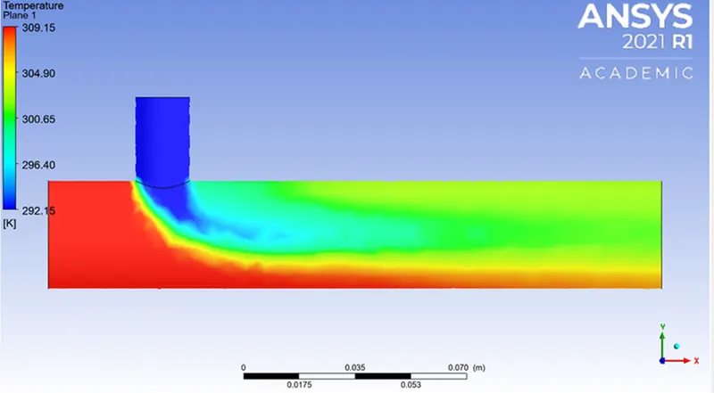
Figure 16: Temperature contour plots on the cut planes along and across the short pipe with momentum ratio 2.

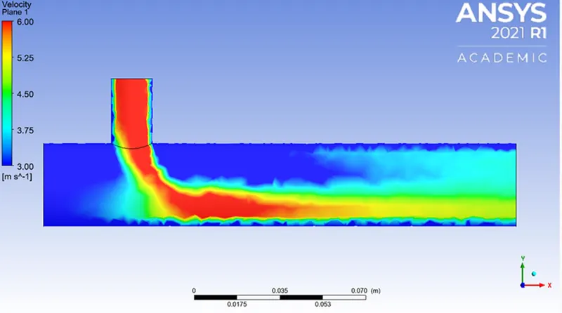
Figure 17: Velocity contour plots on the cut planes along and across the short pipe with momentum ratio 2.

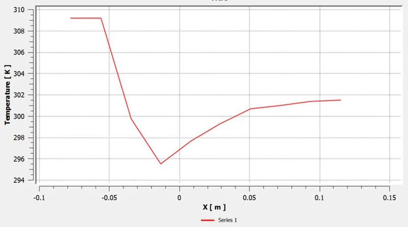
Figure 18: Temperature line plot along and across the length of the short pipe with momentum ratio 2.

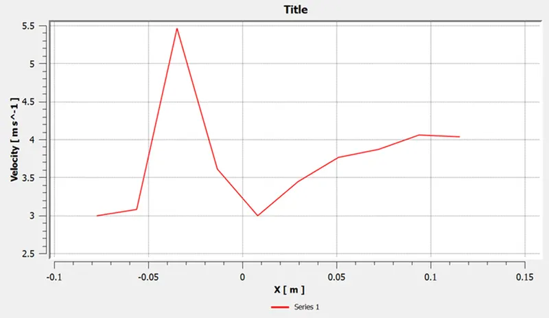
Figure 19: Velocity line plot along and across the length of the short pipe with momentum ratio 2.

b:

Momentum ratio	4
Inlet x velocity	3 m/s
Inlet y velocity	12 m/s
Inlet x temperature	36 C
Inlet y temperature	19 C

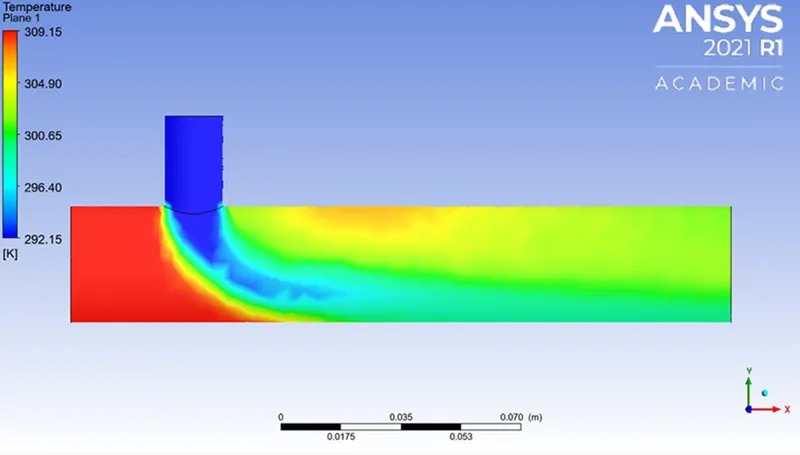
Figure 20: Temperature contour plots on the cut planes along and across the short pipe with momentum ratio 4.

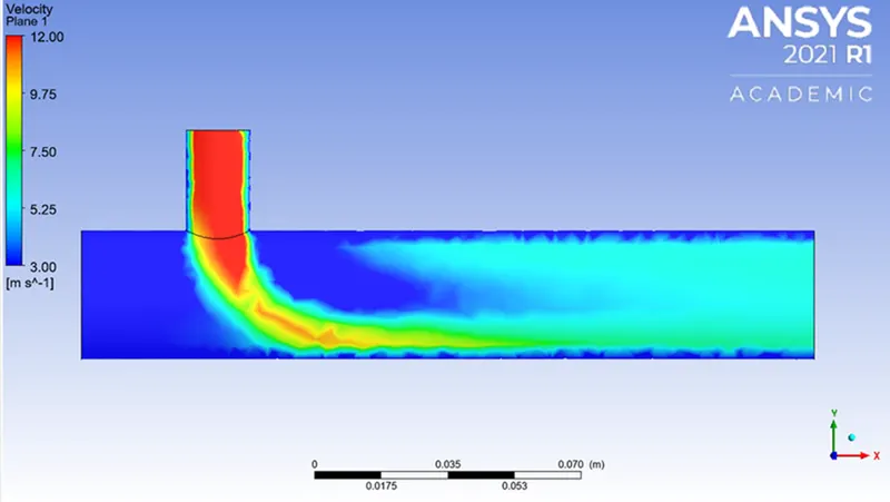
Figure 21: Velocity contour plots on the cut planes along and across the short pipe with momentum ratio 4.

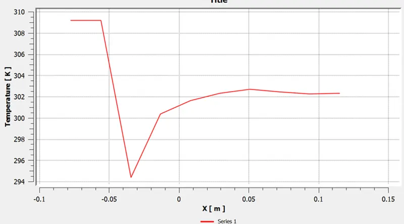
Figure 22: Temperature line plot along and across the length of the short pipe with momentum ratio 4.

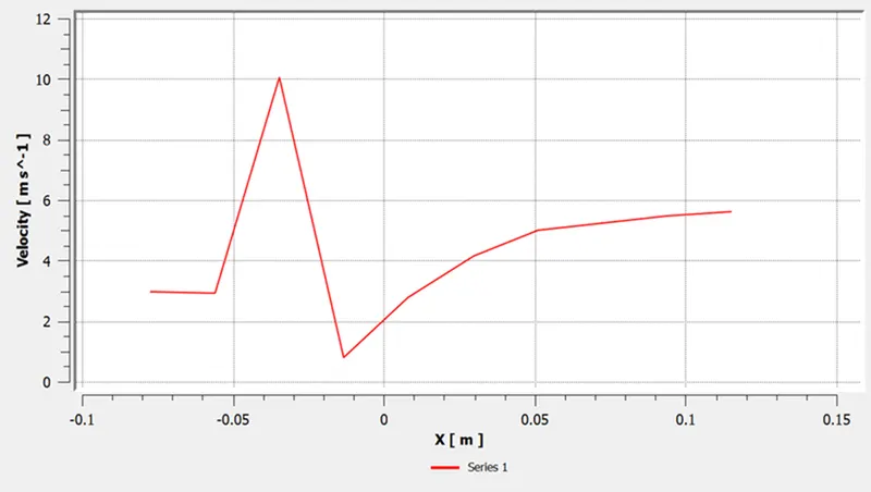
Figure 23: Velocity line plot along and across the length of the short pipe with momentum ratio 4.

Case 2 : Mixing Tee Long

a:

Momentum ratio	2
Inlet x velocity	3 m/s
Inlet y velocity	6 m/s
Inlet x temperature	36 C
Inlet y temperature	19 C

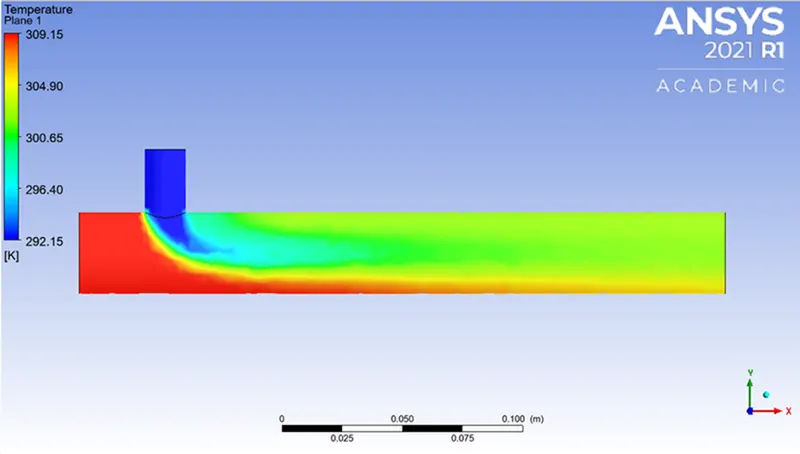
Figure 24: Temperature contour plots on the cut planes along and across the long pipe with momentum ratio 2.

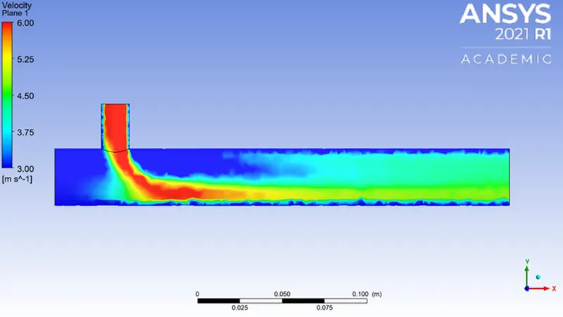
Figure 25: Velocity contour plots on the cut planes along and across the long pipe with momentum ratio 2.

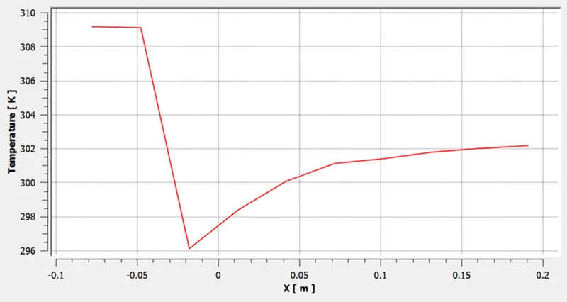
Figure 26: Temperature line plot along and across the length of the long pipe with momentum ratio 2

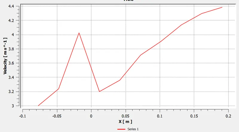
Figure 27: Velocity line plot along and across the length of the long pipe with momentum ratio 2

Case 2 : Mixing Tee Long

b:

Momentum ratio	4
Inlet x velocity	3 m/s
Inlet y velocity	12 m/s
Inlet x temperature	36 C
Inlet y temperature	19 C

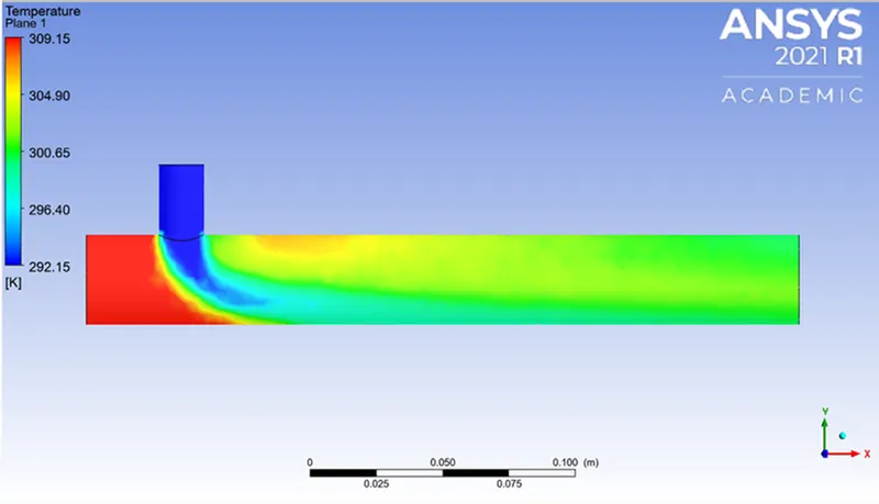
Figure 28: Temperature contour plot on the cut planes along and across the long pipe with momentum ratio 4.

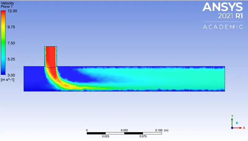
Figure 29: Velocity contour plot on the cut planes along and across the long pipe with momentum ratio 4.

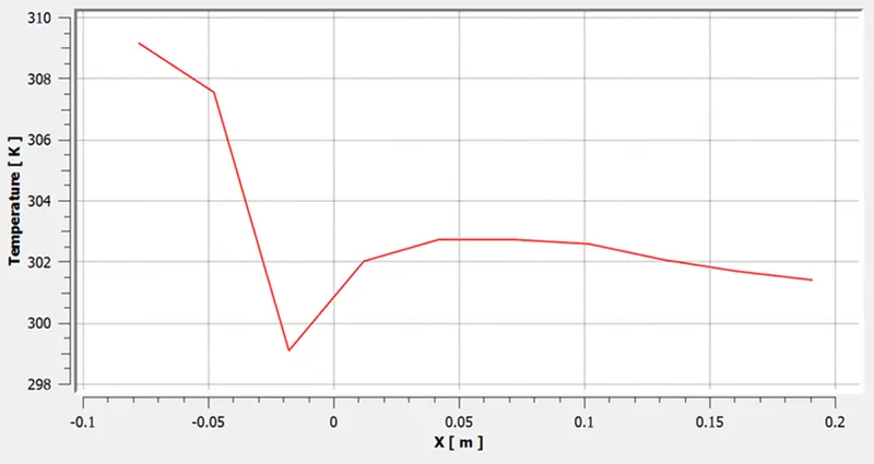
Figure 30: Temperature line plot along and across the length of the long pipe with momentum ratio 4

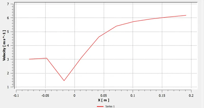
Figure 31: Velocity line plot along and across the length of the long pipe with momentum ratio 4

Case	Momentum ratio	Average temperature (C)	Average velocity (m/s)
Mixing Tee Short	2 4	28.35 29.35	4.11 5.98
Mixing Tee Long	2 4	29 28.35	4.4 6.1

Table 2: Comaprison of average temperature and velocity at outlet for both the models at both momentum ratios.

CONCLUSION

• K-epsilon models suggest flow away from walls, whereas K-omega models predict flow close to walls. The K-epsilon model is used in this scenario because flow near the walls is not taken into account.
• It can be observed that raising the momentum ratio, i.e. inlet velocity, improves the mixing of hot and cold fluids at the output.
• The length of the Tee has no effect on the mixing process because the outlet temperatures and velocities do not change significantly for both momentum ratios.