CFD analysis of Mixing Tee by using Ansys Fluent.
Aim: CFD analysis of Mixing tee by using Ansys Fluent.
Introduction:
Mixing tees—in which two fluid streams with different physical and/or chemical properties mix—are widely used in the petrochemical industry. When there is a large temperature difference between two streams, large metal temperature fluctuations can occur in the region where the two streams meet if proper design steps are not taken. The temperature fluctuations in the metal can lead to thermal fatigue of the pressure boundary piping. If through-wall cracking occurs, the fluid may leak, possibly causing a fire and damage. Therefore, it is imperative to ensure that the piping system can withstand the temperature fluctuations.The given problem is focused in analysing the mixing effectiveness of hot and cold fluid in a tee shaped pipe. A numerical study using CFD approach is applied to predict the outlet temperature and velocity of the pipe at a steady state condition. The computational geometry is modelled using URANS based solver namely k-epsilon and k-omega model. With different momentum ratio, physical parameters like no of iterations, cell count, area weighted average, and standard deviation of temperature at the outlet is predicted. Finally, with different grading of mesh size a grid independence test is conducted to justify the effectiveness of mixing fluids and to measure out the best model for the problem.
Given Data: Hot Inlet Temperature=36 degree C at inlet-x
Cold Inlet Temperature=19 degree C at inlet-y
Hot Inlet velocity for both the cases=3 m/sec.
Momentum ratio= velocity at cold inlet/ velocity at hot inlet, i.e. use this momentum ratios{2,4} respectively.
Problem statement: To compare the mixing effectiveness of TEE joint by using k-omega & k-epsilon model at momentum ratio factor 2,4.
Objectives:
- Execute simulation for short and long TEE model based upon RANS [ Reynolds Averaged Navier stokes] model
- Compare velocity and temperature profiles for both cases. aslo compare cell count, no. of iterations, outlet temperatures.
- Perform gride independence test
- Temperature and velocity plots on cut and across the plane.
Procedure:
- Setup the geometry of model in Ansys workbench.
- Extract the wet volume i.e volume associated by flowing fluid.
- Generate the fine mesh of correct sizing on geometry.
- Set up post processing data & required turbulence model.
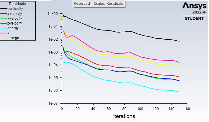
- Run the solver by applying no of iterations and check for the convergence.
- Post process the results by Post CFD.
Turbulence Models:
Most of the CFD problems are based on turbulence modeling, some popular turbulence model applied to the present roblem is discussed below:
K-epsilon model- is the most common model used in computational fluid dynamics (CFD) to simulate mean flow characteristics for turbulent flow conditions. It is a two equation model that gives a general description of turbulence by means of two transport equations (partial differential equations, PDEs). The original impetus for the K-epsilon model was to improve the mixing-length model, as well as to find an alternative to algebraically prescribing turbulent length scales in moderate to high complexity flows.
- The first transported variable is the turbulent kinetic energy (k).
- The second transported variable is the rate of dissipation of turbulent kinetic energy (ε).
k-ε model focuses on the mechanisms that affect the turbulent kinetic energy. The mixing length model lacks this kind of generality. The underlying assumption of this model is that the turbulent viscosity is isotropic, in other words, the ratio between Reynolds stress and mean rate of deformations is the same in all directions.
Realizable k-ε Model: An immediate benefit of the realizable k-ɛ model is that it provides improved predictions for the spreading rate of both planar and round jets. It also exhibits superior performance for flows involving rotation, boundary layers under strong adverse pressure gradients, separation, and recirculation. In virtually every measure of comparison, Realizable k-ɛ demonstrates a superior ability to capture the mean flow of the complex structures.
K-omega SST model-
SST stands for shear stress transport. The SST formulation switches to a k−ϵ behavior in the free-stream, which avoids the k−ω problem of being sensitive to the inlet free-stream turbulence properties. The k−ω SST model provides a better prediction of flow separation than most RANS models and also accounts for its good behavior in adverse pressure gradients. It has the ability to account for the transport of the principal shear stress in adverse pressure gradient boundary layers. It is the most commonly used model in the industry given its high accuracy to expense ratio. On the negative side, the SST model produces some large turbulence levels in regions with large normal strain, like stagnation regions and regions with strong acceleration. This effect is much less pronounced than with a normal k-epsilon model though.
1.Preprocessing setup:
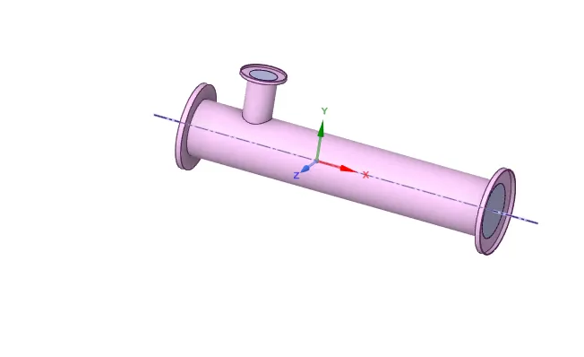
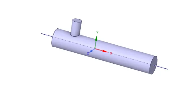
1. Convert the mechanical body of mixing tee into desirable CAD model using ANSYS SpaceClaim. also extract the fluid volume region by selecting edge command from the volume extraction tool at prepare physics section. The solid model is suppressed from the fluid model to crate mesh at region of interest.
2. Mesh Generation:
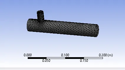
- Wet volume geometry is imported to the workbench.
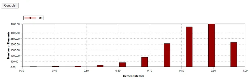
- Hit the statistics option, the no of elements and nodes are highlighted. The mesh metric shows the no of triangular, pyramidal, trapezoidal members required at a certain percentage to optimise the mesh model.
- Define the differents names by Named selection option. i.e., inlet-x, inlet-y, outlet & walls.
- After hitting mesh generation, click on update in order to update the model.
3.Set up of Physics Solver:
- The Fluent solver is launched by double clicking on setup. where the graphics and console plane appear.
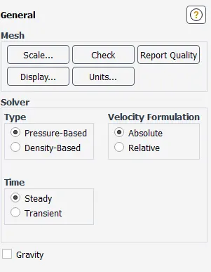
- From the general tab, we can select the pressure-based solver having absolute velocity formation and within a steady state condtion.
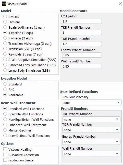
- Click on the energy parameter to activate. then use viscous model to select K-epsilon Realizable or K-omega SST respectively.
- Specify the material as Air.
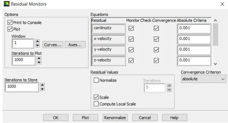
- Define the cell zones condtions and Boundary conditons for inlet-x,inlet-y, wall specifying the inlet temperature and velocity.
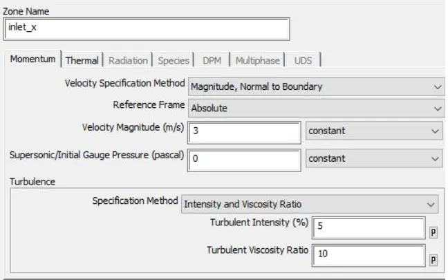
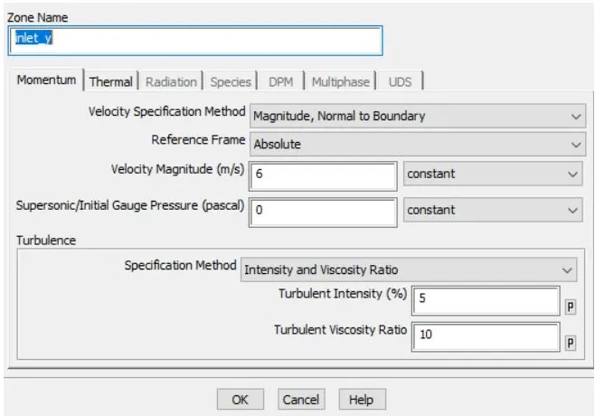
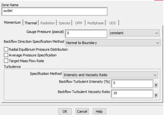
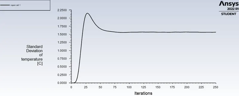
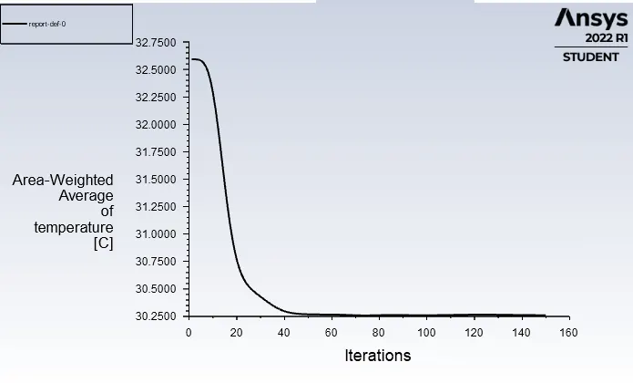
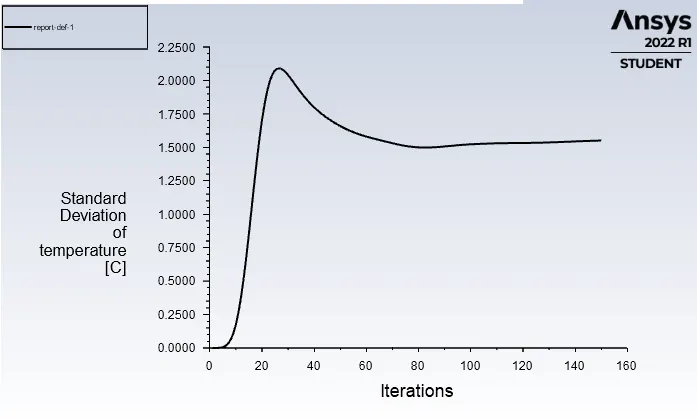
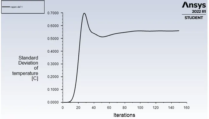
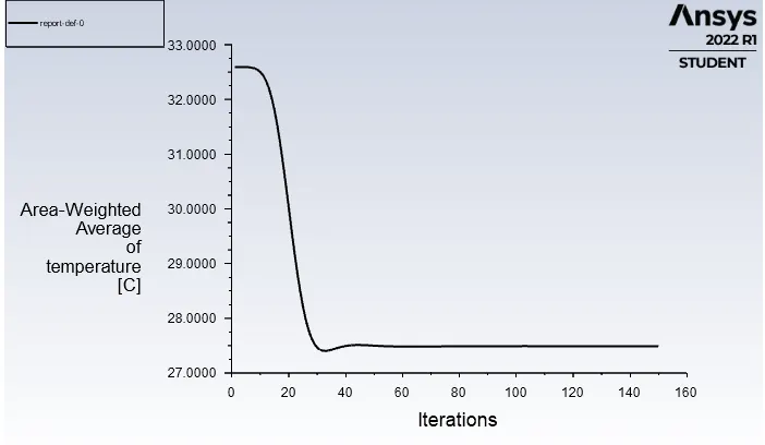
- The monitor setting is specified to two parameters- Area-weighted average and Standard deviation.
- Initialized the solver with hydrid schemes.
- Set up the no of iterations. and hit the calculate option.
4. Post Processing Results:
- After computaion ends check for graphical visualization for the iteration convergence rate, area weighted average temperature and standard deviation plot at outlet section.
- Launch the Post CFD and activate inlet ,outlet, wall sections to view the model.
- select the plane along and across the geometry of model.
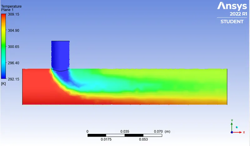
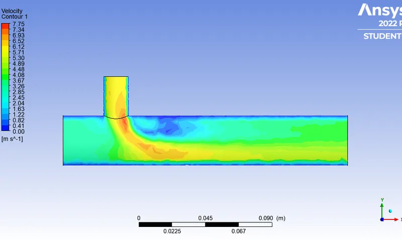
- Highlight the planes with temperature amd velocity variables.
- Use line plot along and across the model and measure the temperature and velocity variations charts.
case1-A SHORT TEE:
MODEL: K-EPSILON
MOMENTUM RATIO: 2
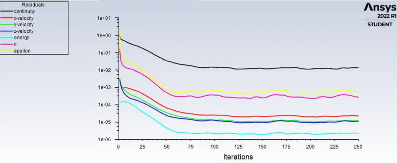
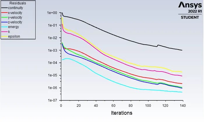
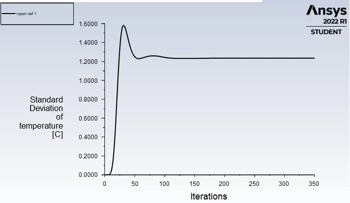
Convergence for iteration: No if iterations required for convergence is:125
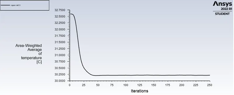
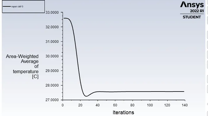
Area-Weighted Average of Temperature:
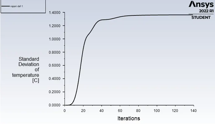
Standard Deviation of Temperature:
5. Post processing Results:
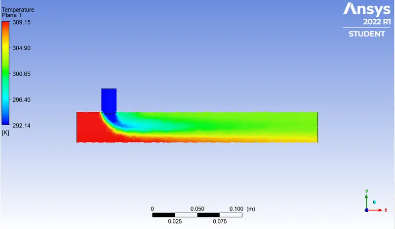
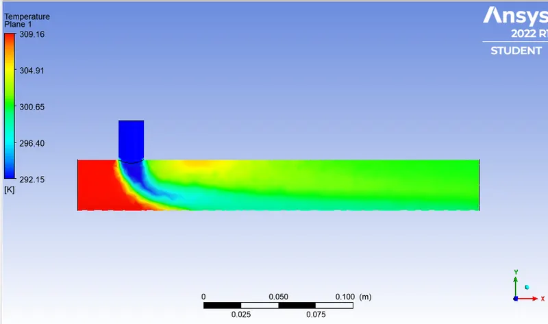
Temperature profile:
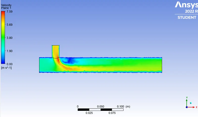
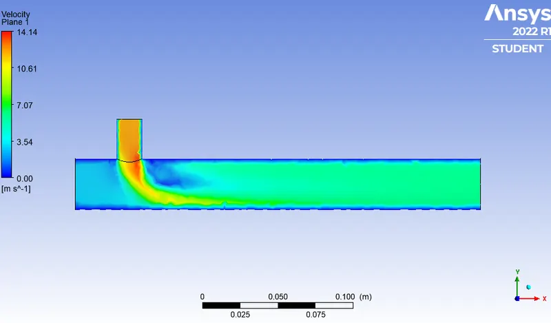
Velocity Profile:
MODEL: K-Omega SST
MOMENTUM RATIO:2
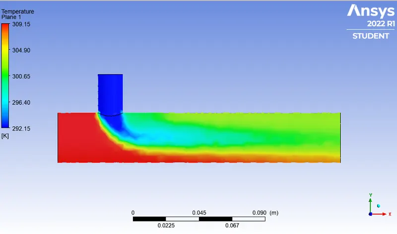
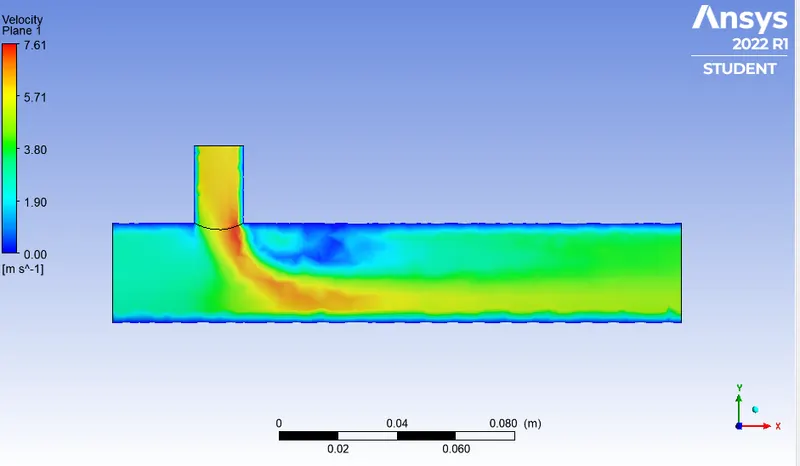
In the above contour, we can see flow differences in K-epsilon and k-omega SST. Let us understand why they are different:,
K-epsilon:
- K-epsilon turbulence model is the most commonly used model in CFD to simulate the mean flow characteristics for turbulent flow conditions. It is a two-equation model that gives a description of turbulence by means of two transport equations (PDE's). The first transport variable is turbulent kinetic energy and the second transport variable is the rate of dissipation of turbulent kinetic energy.
- k-epsilon focuses on the mechanism that affects the turbulent kinetic energy.
K-Omega SST:
- k-omega SST is a two-equation eddy viscosity model that is used for many aerodynamics applications. It is a hybrid model combining the Wilcox omega and k-epsilon models. A blending function activates the Wilcox model near the wall and k-epsilon in the free stream. This ensures that the appropriate model is utilized through the flow field.
Main Difference:
- K-omega model is well suited for simulation flow in the viscous sub-layer. On the other hand, k-epsilon is idealing for predicting flow in the regions away from walls.
- The K-omega exhibit less sensitivity to the free stream conditions than any other turbulence models.
In this particular case we are not dealing with walls, therefore we are going to use the K-epsilon method for further simulation.
Case1-B Short Tee: model: K-epsilon
Inlet velocity- 3m/sec,
momentum ratio:4
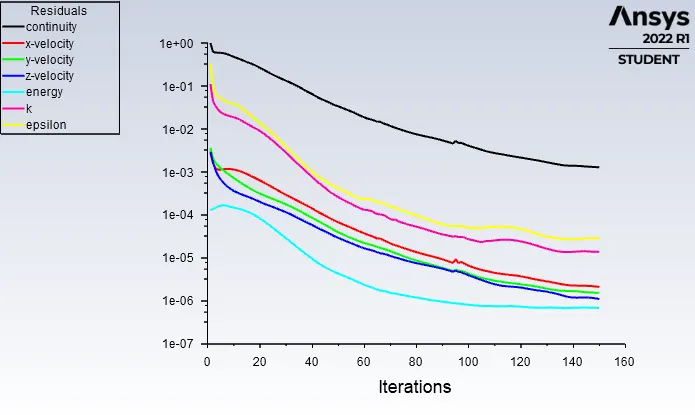
convegrence Plot
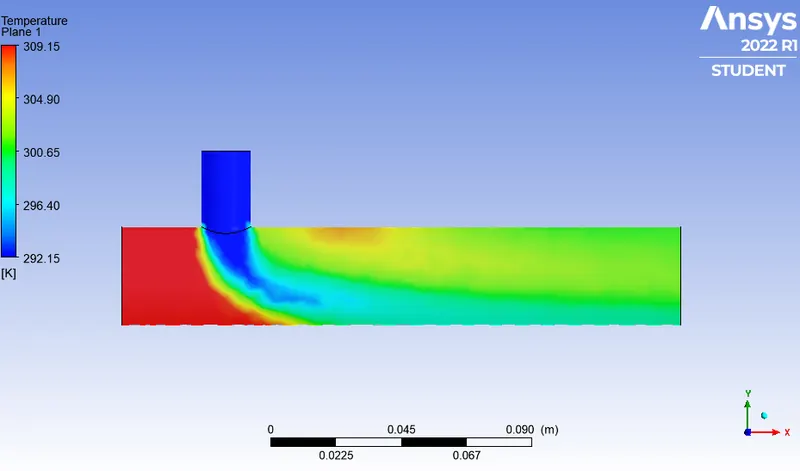
Temperature contour:
Velocity contour:
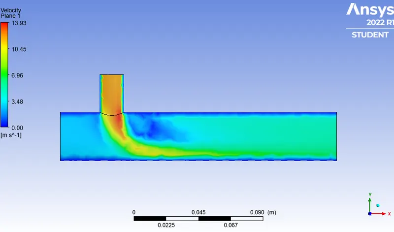
Case2 Long Mixing Tee:
Momentum ratio:2
Inlet velocity: 3m/sec
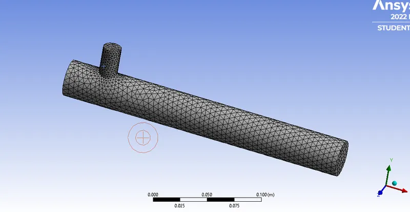
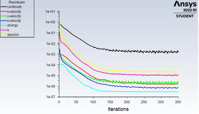
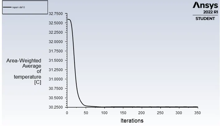
Case2-B Long Mixing Tee:
Momentum Ratio:4
Inlet Velocity: 3m/sec
Comparison between both the turbulent model for different geometry with analytical solution.
K-EPSILON MODEL
| Geometry | Momentum Ratio | Cell Count | Avg outlet Temp | No. of Iterations |
| Short Tee | 2 | 12780 | 30.25 | 135 |
| Short Tee | 4 | 12780 | 27.20 | 139 |
| Long Tee | 2 | 15727 | 30.25 | 125 |
| Long Tee | 4 | 15727 | 27.58 | 150 |
Mesh Independence Test:
- Mesh independence or Grid independence study is something we can perform to determine the dependence of the results on the mesh density.
- Compare the results for various runs for different sizing of the meshing elements. In order to pass, mesh independence results should obtain with proper precision.
Conclusion:
- The K-epsilon model is seen to br effective in capturing the physics of thermal and flow behaviour starting from entry to outlet.
- The k-epsilon model predicts flow virtually far from the boundaries and the k-omega model predicts near the walls. As for this case we required a flow simulation turbulent model far from the walls,so we have used k-epsilon model respectively.
- After conducting simulations, as element number increases the convergence time also increases.
- To get better mixing at outlet high velocity of flow is very effective. Therefore, a higher momentum ratio gives better mixing of hot and cold fluid streams at the outlet.
- Finally, in the above case, it is very important to use a short mixing tee with a momentum ratio of 4, aslo [2 times velocity at inlet-y] to get best results.