Week 1- Mixing Tee
Aim :
To set up steady-state simulations to compare the mixing effectiveness when hot inlet air temperature is 360C & the Cold inlet air is at 190C.
Objective :
Case 1
- Short mixing tee with a hot inlet velocity of 3m/s.
- Momentum ratio of 2, 4.
Case 2
- Long mixing tee with a hot inlet velocity of 3m/s.
- Momentum ratio of 2, 4.
Use the k-epsilon and k-omega SST model for the first case and based on your judgment use the more suitable model for further cases.
Momentum ratio = velocity at cold inlet / velocity at hot inlet.
Theory :
Mixing Tee
- A mixing Tee is formed by two pipe sections joined at a right angle to each other.
- One stream passes straight through the Tee while other enters perpendicular at one side.
- These are used in blending of some oils(injection of additives) and petro-chemical products.
- Blending of fuel gas and mixing of feed streams for catalytic reactors.
- These are having applications in HVAC system .
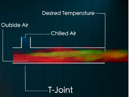
- As far as this challenge is considered , here we are taking two mixingTee i.e, one is short and other is long .In the X-direection ,the hot outside air is flowing and in vertical Y-direction, the cold air stream enters and results in mixing of same .In an accordance with that the desired temperature is obtained at the outlet.
- To study the effectiveness of mixing , a standard deviation plot graph is plotted in surface monitor at solution section of ansys fluent.
- In order to capture the turbulence and mixing ,we are taking the k-epsilon and k-omega turbulence model.
- Different momentum ratio is taken so that the outlet temperature variation is studied.
- k-epsilon is widely applied turbulence model base onpartial differential equations for the turbulent kinetic energy 'k' and its dissipation rate 'epsilon'.
- As far as turbulence is considered ,it is characterised by eddies with different space and time scales.Turbulence brings better mixing of a fluid and produces an additional diffusive effect. Such diffusion is known as eddy diffusion.
- At large Reynolds number there exists a continous transport of energy from large eddies to small eddies .Near the wall ,small eddies destroy themselves in dissipating energy i.e, converting kinetic energy of eddies into inter-molecular energy.
- In this problem , the fluid coming with high velocity(cold fluid) mixes with hot fluid ,the energy diffuses and mixing taking place and also momentum transfer due to velocity variation enables turbulence downstream of the mixing point.
Procedure :
Step 1 : Geometry (pre-processing)
After selecting the Geometry startclaim is going to start It is a software to create CAD designs for CFD and FEA.
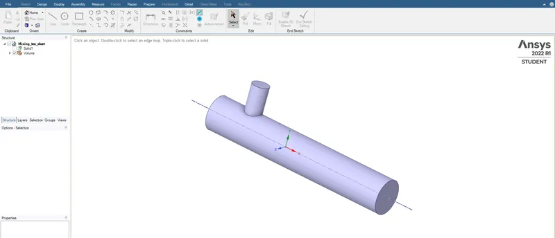
After that we have to extract the fluid area where the fluid flows go to prepare and select the Volume Extract by selecting the edges of the geometry and Then hide and supress for Physics the solid model, It means it is not going to loaded when we are doing the simulation process.
Step 2 : Mesh
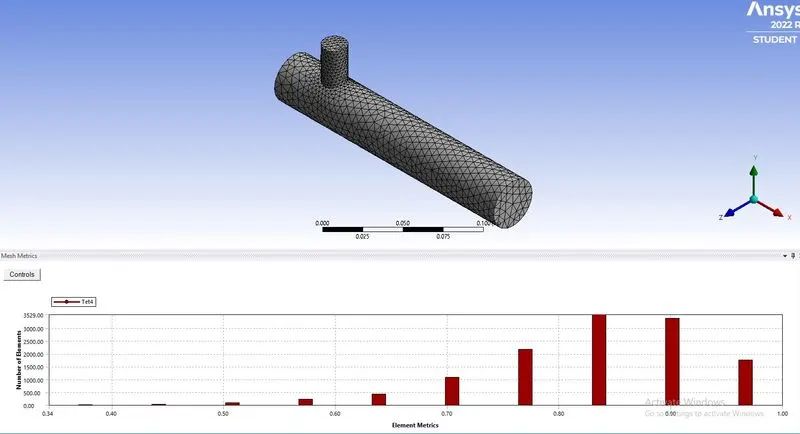
When the Mesh Software has started first we have to create the names of the geometry by Named selection command Select by edges name given in this project are inlet x, inlet y, outlet and walls. After this we are generating mesh and the default mesh size is around mm and we are check the mesh quality
Step 3 : Setup and Solutions
Start the setup launching the Fluent In this you have to check the mesh updated or not After opening the fluent First we have to setup for physics - In this case we are solving for steady state for small mach number- pressure based solver. Velocity formulations is absolute and for Temperature energy equation we are using.
For Turbulence model in the viscous section you can use the K- Epsilon and K-omega models as per the equations. Now, we are going to add the boundaries values like Velocity and Temperature for the geometry like inlet velocity and inlet Temperature etc.
After that In the case we are going to calculate the average temperature at Outlet and standerd deviation for mixing effectiveness of the two fluids at T section by the solution you can get the reports and then initilase the initial conditions and after that hit the calculation we got these reports mentioned below.
Case 1 : Short mixing tee
A) For both the models k- Epsilon and k-omega and momentum ratio = 2 where the hot inlet velocity is 3 m/s and cold inlet velocity 6 m/s.
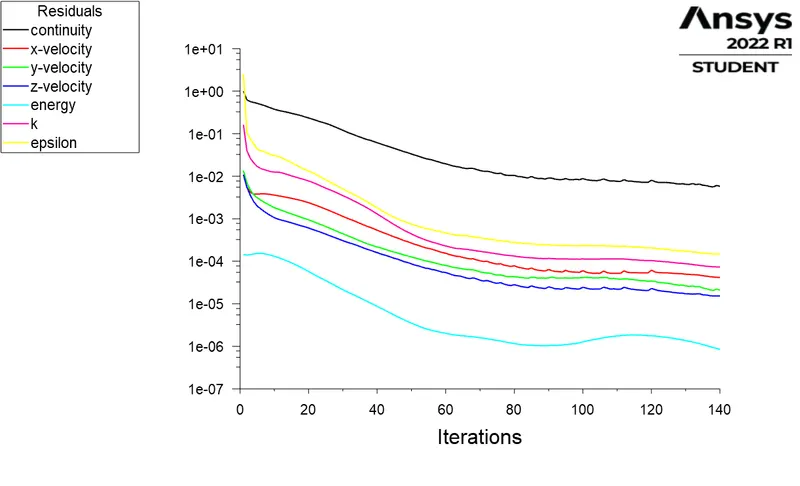
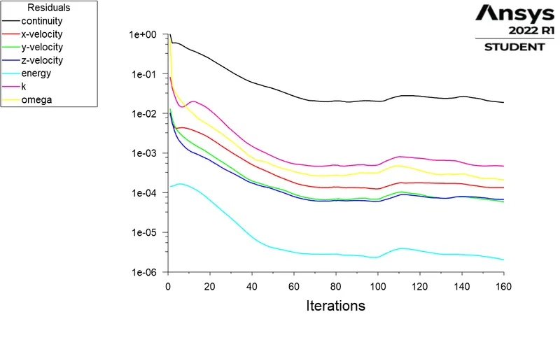
1. Residual graphs - to check the solution how much numerically accurate
- K-epsilon model :
- K-omega model :
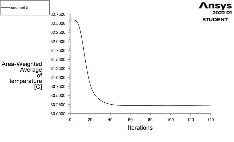
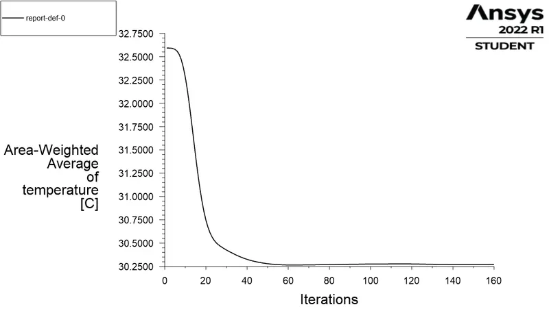
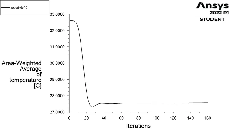
2. Area - weighted Average of Temperature - to get the average outlet temperature.
- K-epsilon model :
- K-omega model :
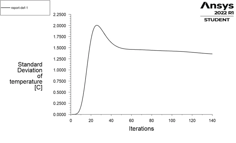
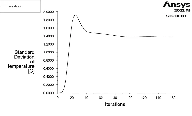
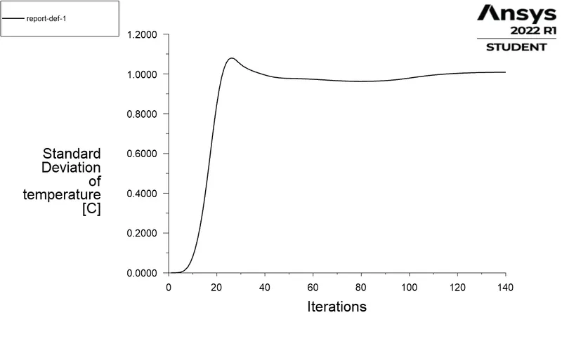
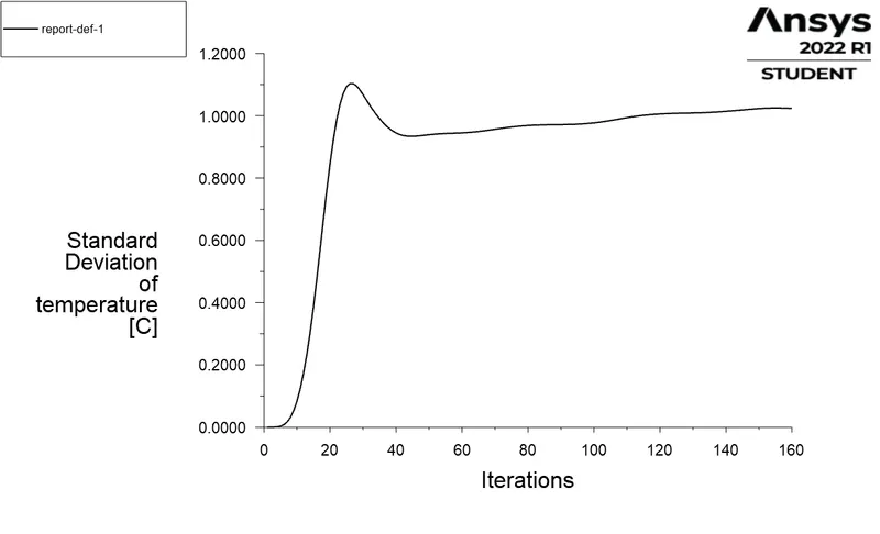
3. Standard Deviation plot - to understand the effectiveness of mixing.
- K-epsilon model :
- K-omega model :
B) For both the models k- Epsilon and k-omega and momentum ratio = 4 where the hot inlet velocity is 3 m/s and cold inlet velocity 12 m/s.
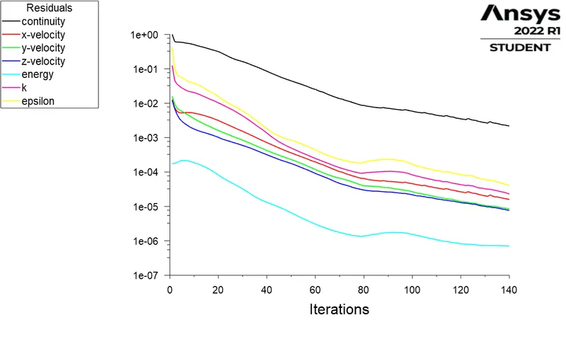
1. Residual graphs - to check the solution how much numerically accurate
- K-epsilon model :
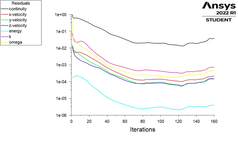
- K-omega model :
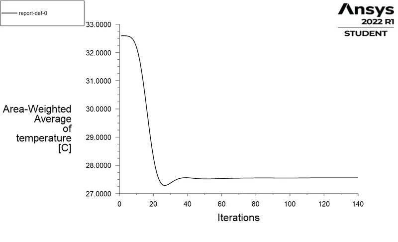
2. Area - weighted Average of Temperature - to get the average outlet temperature.
- K-epsilon model :
- K-omega model :
3. Standard Deviation plot - to understand the effectiveness of mixing.
- K-epsilon model :
- K-omega model :
Observations :
- In these plots we can clearly see the there is minimum difference between them but In the residual graph you can clearly see the k Epsilon model after some value the solution coverges and the plot becomes uniform.
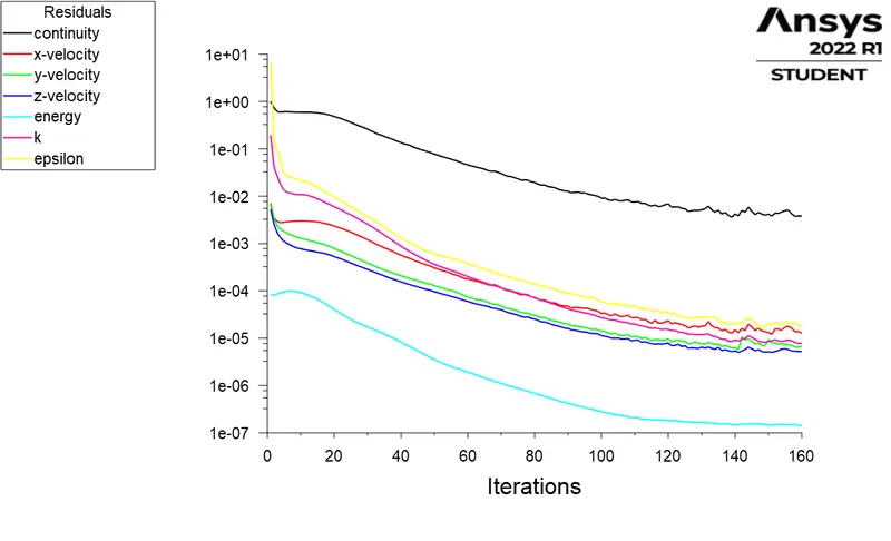
- The residual plot always shows downward slope or decreasing line means the lower the residual value is the more numerically accurate the solution.
- The residual plot of momentum ratio =4 are more uniform means there is no significant diffrence errors to got the converged solution as compared the momentum ratio 2 the value is still 1e-6.
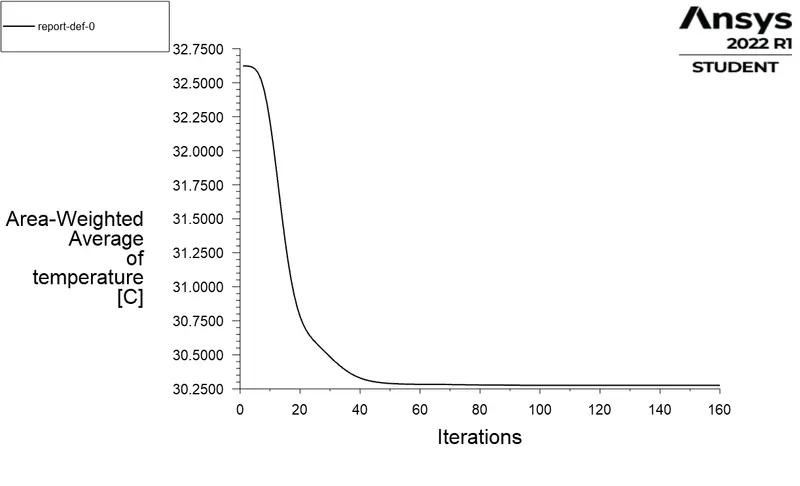
- In the section where the inlet hot or inlet cold fuilds mixes the temperature is get high for some seconds and after that we got uniform average outlet temperture.
- In these graphs we can clearly see that after increasing the velocity its not seem steady or uniform as compared the momentum ratio 2 as standered deviation is low we got the uniform temperature.
- K-Epsilon model predicts well far from the boundaries or walls and k - omega model predicts well near walls. Even though it depends on Y+. We also use SST model which is a combination of these.
- K-epsilon model shows standerd results because it becomes uniform after certain value So, in this case we are going to use K-epsilon model.
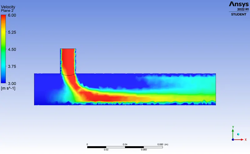
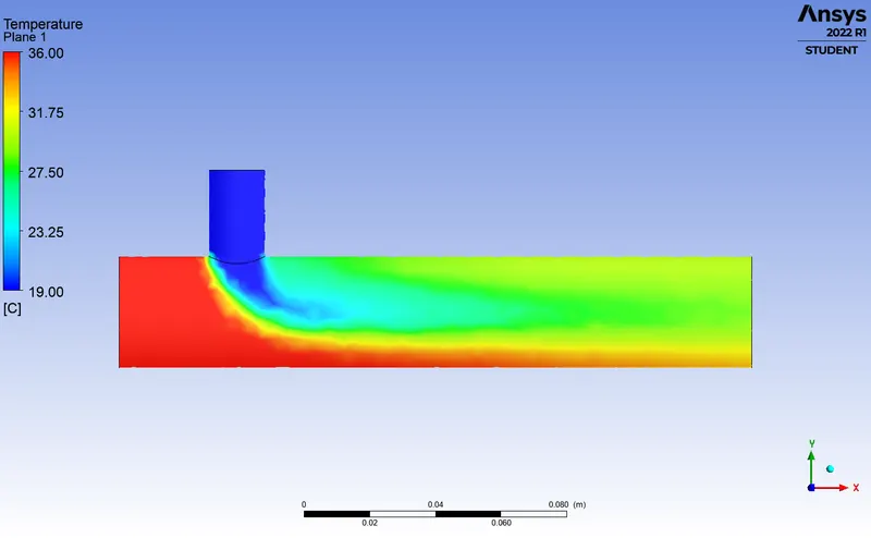
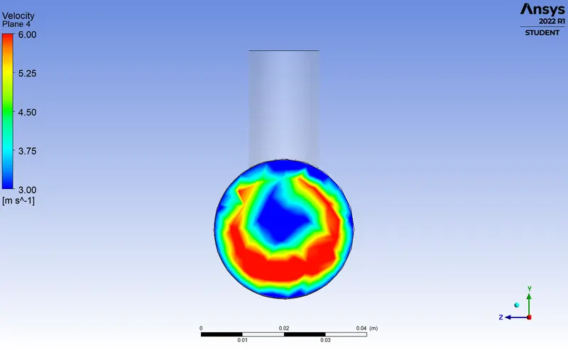
Velocity and temperature contour plots on the cut planes along the pipe :
- Velocity distribution :
- Temperature distribution :
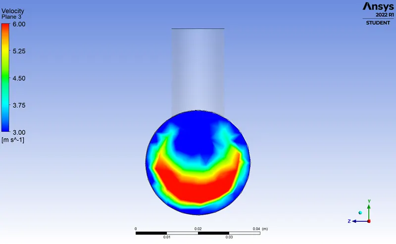
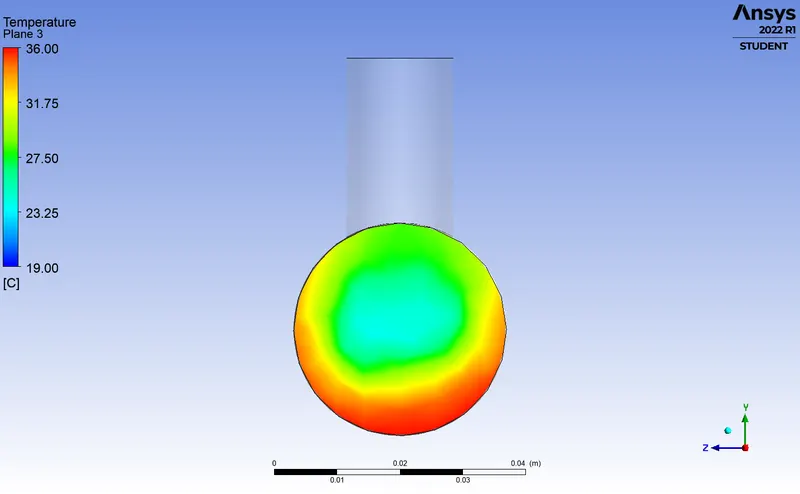
Velocity and temperature contour plots on the cut planes across the pipe :
- Velocity distribution :
- Temperature distribution :
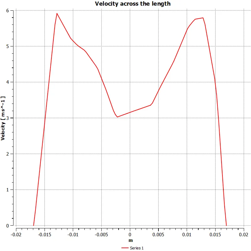
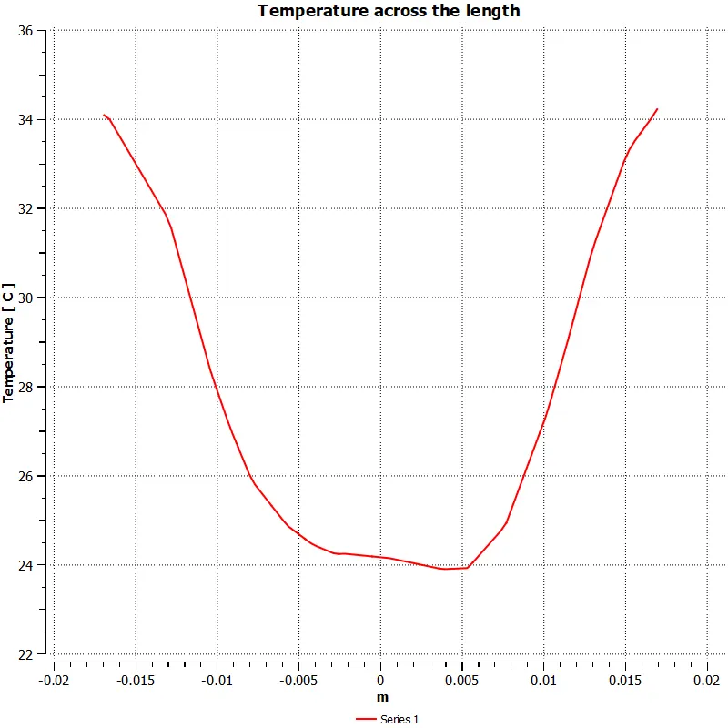
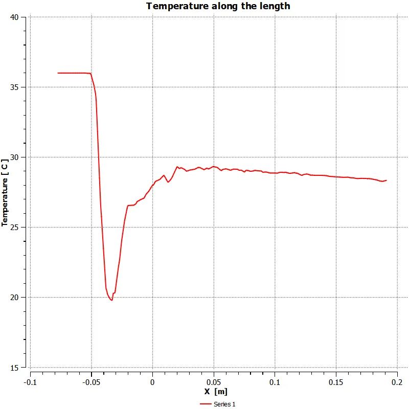
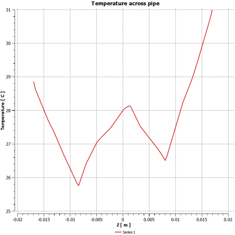
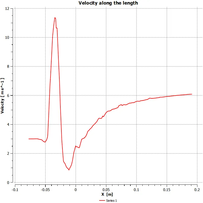
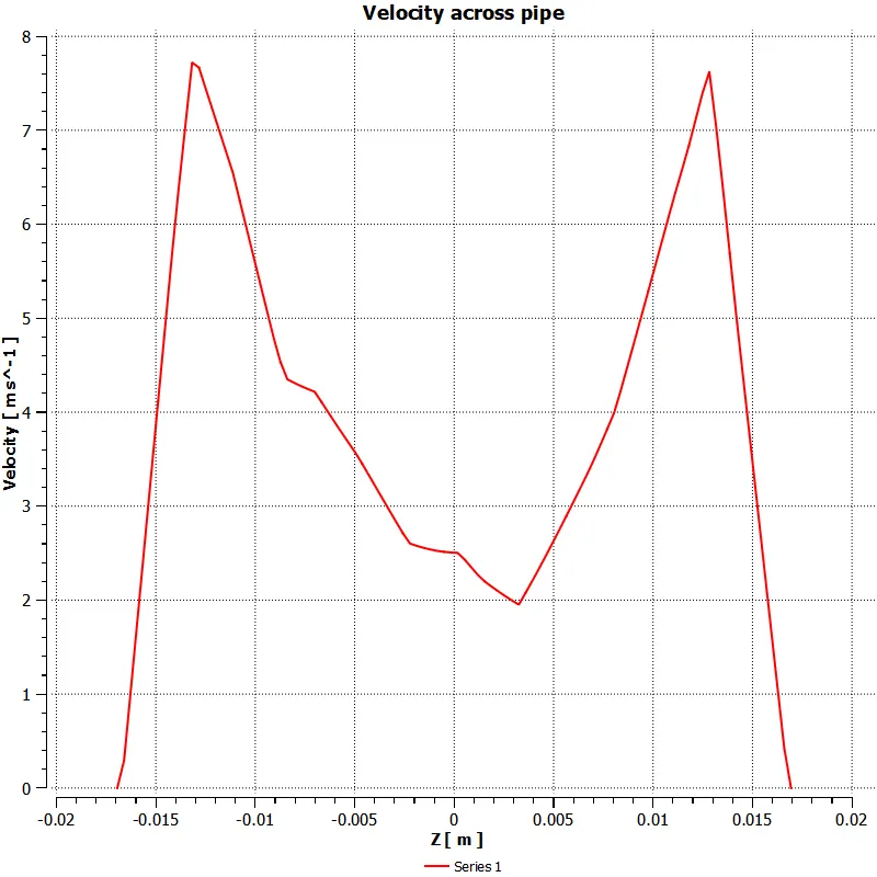
Velocity and temperature line plots across the length of the pipe :
- Velocity distribution :
- Temperature distribution :
Case 2 : Long mixing tee
A) For both the models k- Epsilon and k-omega and momentum ratio = 2 where the hot inlet velocity is 3 m/s and cold inlet velocity 6 m/s.
1. Residual graphs - to check the solution how much numerically accurate
- K-epsilon model :
- K-omega model :
2. Area - weighted Average of Temperature - to get the average outlet temperature.
- K-epsilon model :
- K-omega model :
3. Standard Deviation plot - to understand the effectiveness of mixing.
- K-epsilon model :
- K-omega model :
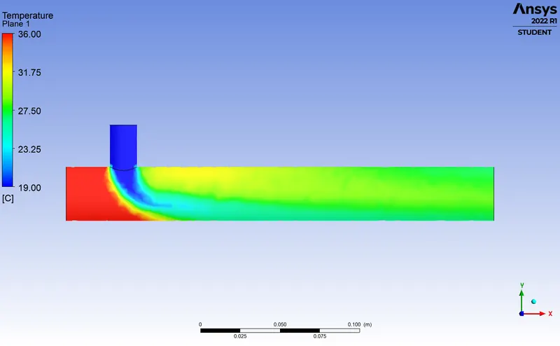
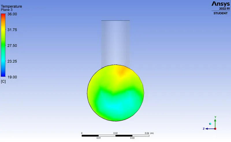
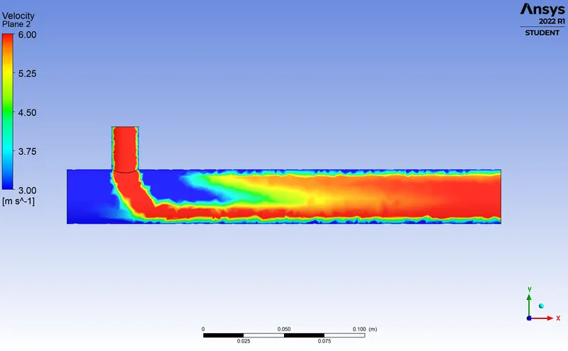
Velocity and temperature contour plots on the cut planes along and across the pipe :
- Temperature distribution :
- Velocity distribution :
Velocity and temperature line plots along and across the length of the pipe :
- Temperature distribution :
- Velocity distribution :
Comparison between two cases - Short mixing tee and Long mixing tee
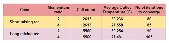
Effect of length and momentum ratio on results :
- From the above calculation we can clearly conclude that there is no difference in the outlet temperature means outlet temperature is independent of length.
- But, Momentum ratio effects the Outlet temperature by increasing the momentum ratio the outlet temperture is dropping or decresing.
- By increasing the momentum ratio the errors of residuals are increasing means it is going to effect the numerically accurance of the solution.
Mesh independent study :
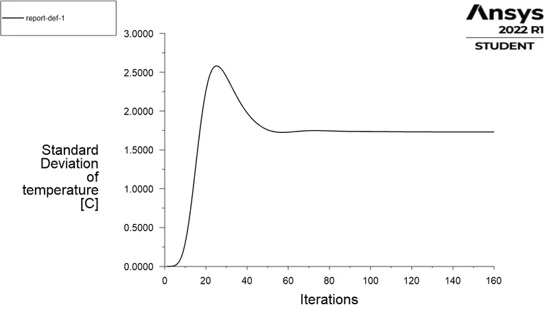
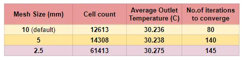
In the CFD we have to solve the Governing equations of Fluid dynamics for each cells So, the more cells the more equations we have to solve and that's why it takes time in simulations as per increment in the cell counts.The more the mesh size the cell count number is less and when you decrease the mesh size the cell count is more So, each and every increment of mesh cells you get converged solution means your standerd deviation of outlet temperature should reach to steady value as you progressively refining the mesh.
It occurs at a particular tolerance and when it is happens your solution is said to be grid converged.
We are going to do Mesh Independent Test for momentum ratio = 2 K-Epsilon Turbulence Model
Mesh generation and mesh quality :
- Element size = around 10mm (default)
- Element size = 5 mm
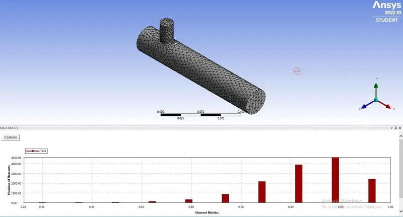
- Element size = 2.5 mm
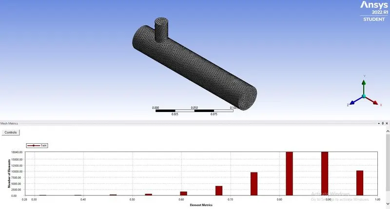
We can easily conclude that these pictures how the mesh size increses and the number of cell counts in the geometry will increses. When we increase the number of cells the simulation time increses quadratically way as well. As you add more number of cells your solver take more iterations to converge a particular value whereas, If the mesh is coarse (means few cells) the linear solver converges very fast.
Residual graph :
- Element size = 10 mm
- Element size = 5 mm
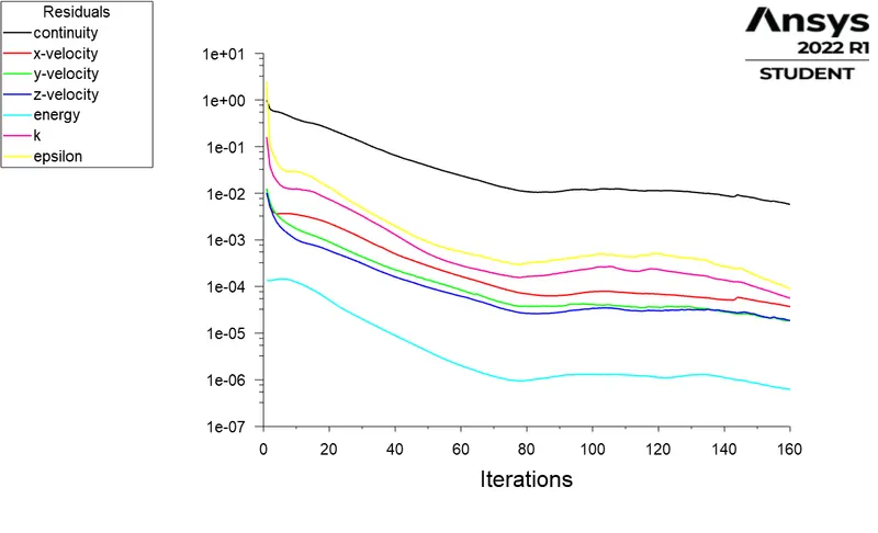
- Element size = 2.5 mm
Area-weighted average of temperature :
- Element size = 10 mm
- Element size = 5 mm
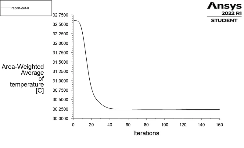
- Element size = 2.5 mm
Standard deviation of temperature :
- Element size = 10 mm
- Element size = 5 mm
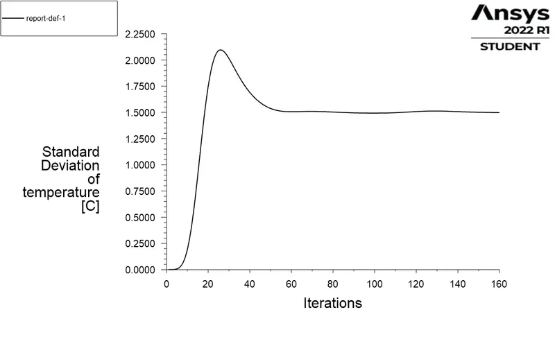
- Element size = 2.5 mm
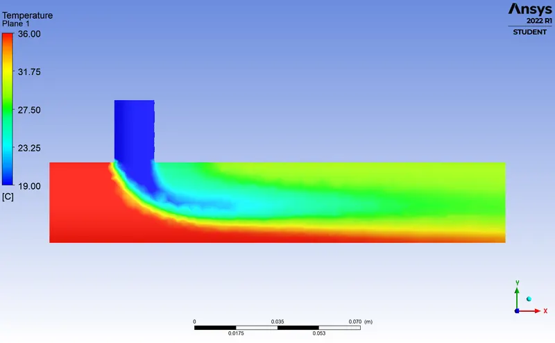
Temperature distribution along length :
- Element size = 10 mm
- Element size = 5 mm
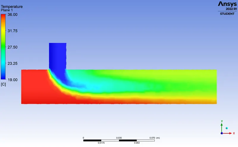
- Element size = 2.5 mm
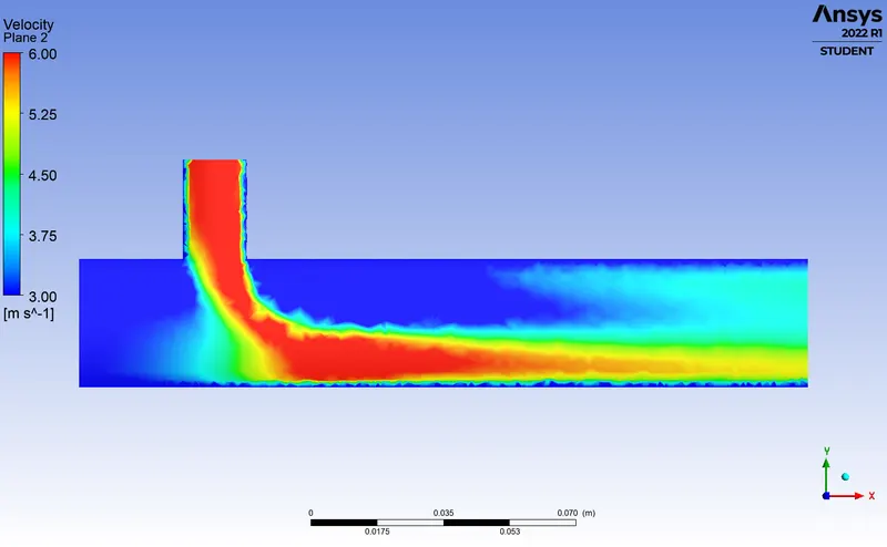
Velocity distribution along length :
- Element size = 10 mm
- Element size = 5 mm
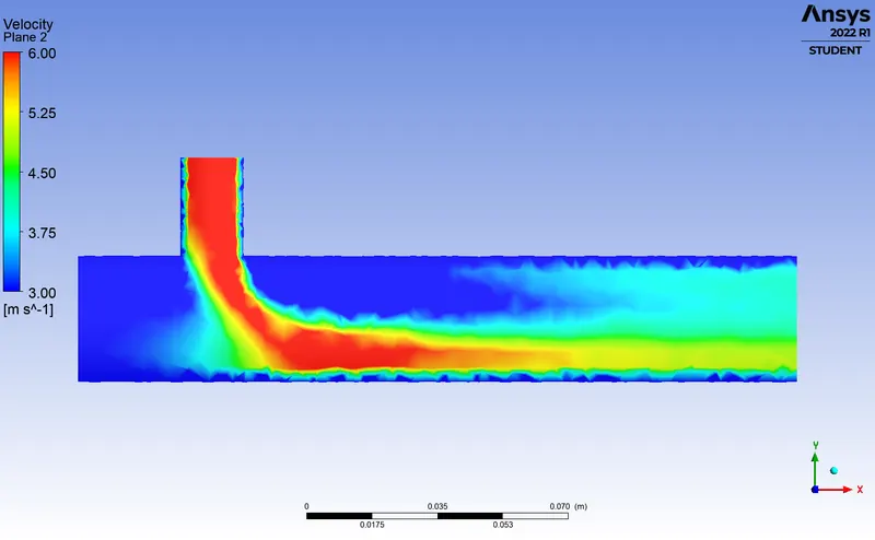
- Element size = 2.5 mm
Comparison between different mesh sizes for case 2 - Short mixing tee
Conclusion :
From this project we can conclude that Temperature drops significantly due to increament in the velocity of cold fluid from the inlet and this is because of the hot and cold fluid meets at the T section and due to the high velocity of cold fluid flow is turbulent or we can say that turbulent mixing we got.
The temperature contour plots for short tee case shows that some high temperature flow without properly mixing at the tee section as compared in the long tee temperature contour plots shows high temperature mixing the rest flow throughly or properly. Therefore, we recomanded long tee high velocity for applications because in this low standered value means temperature is uniform.