Week 1- Mixing Tee

Aim: To set up steady-state simulations to compare the mixing effectiveness when hot inlet temperature is 36⁰C & the Cold inlet is at 19⁰C, for the provided geometries of Short mixing tee and Long mixing tee .

1. Use the k-epsilon and k-omega SST model for the first case and investigate the more suitable model for further cases and state the reason for choosing a suitable model

2. To Compare results for the both cases as given below,

   Case 1:
   Case 1-a : Short mixing tee with a hot inlet velocity of 3m/s and Momentum ratio of 2.
   Case 1-b : Short mixing tee with a hot inlet velocity of 3m/s and Momentum ratio of 4.  

   Case2:
   Case 2-a : Long mixing tee with a hot inlet velocity of 3m/s and Momentum ratio of 2.
   Case 2-b : Long mixing tee with a hot inlet velocity of 3m/s and Momentum ratio of 4. 

              where,
           Momentum ratio = velocity at cold inlet / velocity at hot inlet

    Table of comparison for the following values from the both cases.

• Cell count
• Average outlet temperature
• Number of iterations for convergence

Expected results:

1. Velocity and temperature contour plots on the cut planes along and across the pipe.
2. Velocity and temperature line plots along and across the length of the pipe.
3. The convergence plot for each simulation. 
4. Perform Mesh independent study for any one case.
5. Discuss the effect of length and momentum ratio on results. 

Objective: To simulate the given cases with air as working fluid  in Ansys Fluent and to compare the obtained results with analytical results. Draw the conclusion based on the comparison study.

Given Data:

     Temperature of Hot air (`T_h`) `= 36 ^@ C ` .
     Temperature of Cold air (`T_c`) `= 19 ^@ C ` .
     Desity of air (`rho`) `= 1.225 "kg"/m^3 ` .

     Diameter of Hot air inlet pipe (`D_h`) `= 0.0338781 m ` .
     Diameter of Cold air inlet pipe (`D_c`) `= 0.0169626 m ` .
     Diameter of Mixed air outlet pipe (`D_o`) `= 0.0338761 m ` .

• Cross sectional area of Hot air inlet (`A_h`) `= pi.(0.0338781)^2/4 `
                                                                 ` = 9.013138 xx 10^(-4)  m^2 `.
• Cross sectional area of Cold air inlet (`A_c`) `= pi.(0.0169626)^2/4 `
                                                                  ` = 2.259823 xx 10^(-4)  m^2 `.
• Cross sectional area of Mixed air Outlet (`A_o`) `= pi.(0.03338781)^2/4 `
                                                                       ` = 9.013138 xx 10^(-4)  m^2 `.   
• For Case 1-a  & Case 2-a ,
  Velocity at cold inlet (`V_(ca)`) = Momentum Ratio  x velocity at hot inlet (`V_h`)  `= 2 xx 3 = 6  m/s ` .
   
• For Case 1-b  & Case 2-b ,
  Velocity at cold inlet (`V_(cb)`) = Momentum Ratio  x velocity at hot inlet (`V_h`)`= 4 xx 3 = 12  m/s ` .
   
• Mass flow rate of Hot air for all cases  ,
  `dotm_h = rho xx A_h xx V_h = 1.225 xx 9.013138 xx 10^(-4) xx 3 = 0.003312 "kg/s" `.
  
  
• Mass flow rate of Cold air for Case 1-a and Case 2-a ,
  `dotm_(ca) = rho xx A_c xx V_(ca) = 1.225 xx 2.259823 xx 10^(-4) xx 6 = 0.001661 "kg/s" ` .
  
  
• Mass flow rate of Cold air for Case 1-b and Case 2-b ,
  `dotm_(cb) = rho xx A_c xx V_(cb) = 1.225 xx 2.259823 xx 10^(-4) xx 12 = 0.003322 "kg/s" `.
  
  
• For Case 1-a  & Case 2-a ,
  Velocity at Mixed outlet (`V_(oa)`) `= (dotm_h + dotm_(ca))/ (rho* A_o) = 0.005007 / (1.225 xx 9.013138 xx 10^(-4) ` `=  4.504353 m/s ` .
   
• For Case 1-b  & Case 2-b ,
  Velocity at Mixed outlet (`V_(ob)`) `= (dotm_h + dotm_(cb))/ (rho* A_o) = 0.006676 / (1.225 xx 9.013138 xx 10^(-4)` ` =  6.008705 m/s ` .
  
  
• For Case 1-a  & Case 2-a ,
  Temperature at Mixed outlet (`T_(oa)`) `= ((dotm_h xx T_h) + (dotm_(ca) xx T_c))/ (dotm_h + dotm_(ca)) = ((0.003312 xx 36) + (0.001661 xx 19)) / ((0.003312 + 0.001661) ` `=  30.322382  ^@ C ` .
   
• For Case 1-b  & Case 2-b ,
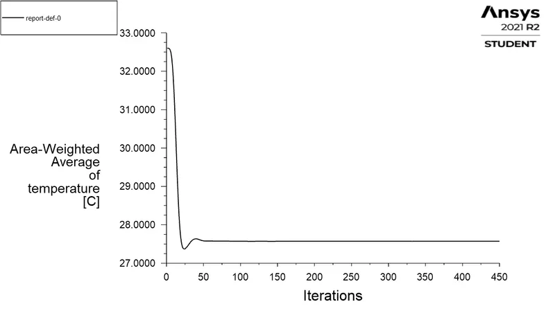
  Temperature at Mixed outlet (`T_(ob)`) `= ((dotm_h xx T_h) + (dotm_(ca) xx T_c))/ (dotm_h + dotm_(ca)) = ((0.003312 xx 36) + (0.003322 xx 19)) / ((0.003312 + 0.003322) ` `=  27.487685  ^@ C ` .

Workflow:

• Open Ansys Workbench and drag and drop Fluid flow (Fluent ) setup from the list into the Project Schematics. Rename it according the case.
• Double click on Geomerty to open the Spaceclaim tool. In spaceclaim import the respective geometry and extract the fluid volume on which the simulations to be performed.
• Check the area and length along with other paremeters of geometry, save the spaceclaim file and close the spaceclaim. 
• In project schematics update the geometry if not already updated automatically. Then double click on mesh to open the ansys meshing tool where mesh is to be generated.
• In the meshing tool geometry will be automatically loaded check and inspect the geometry wether right geometry is loaded. Give the nomenclature to the variuos faces and zones with Named selection. (N is the shorcut key for the same).
• After that generate the desired mesh as per the requirements. Once the mesh has been generated exit the Meshing tool. Update the mesh section under fluent setup in the project schematics if not already updated.
• Double click on setup section to the setup the case for fluent simulation. Where the geometry and mesh will be automatically loaded. Set the general settings for type of simulation, type of solver etc. Under physics tab set the desired models for simulation, select materials or working fluids, cell the cell zones and boundary conditions. For these simulations enable the energy model and under viscous models select k-epsilon or k-omega tubulance models as per the case. 
• Under solutions tab set the settings for convergence and reports. Then initailise the solution by clicking on the initialize button. Set the number of iterations to be performed and click on calculate button to run the simulation. While simulating observe the reports. 
• Once the simulation is finished close the fluent setup and update in the project schematics.
• Double click on results to post process the simulation results. Plot the desired contours and graphs.    

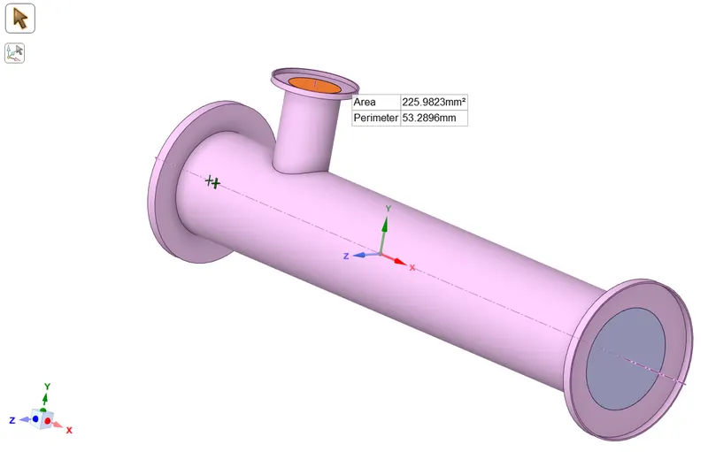
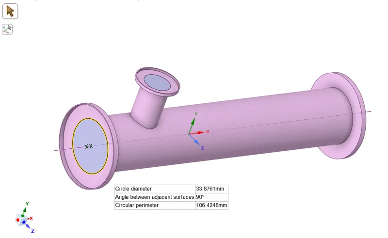
Short Mixing Tee Geometry:

Short Mixing Tee Geometry & Cold inlet area		Short Mixing Tee Geometry & Hot inlet area
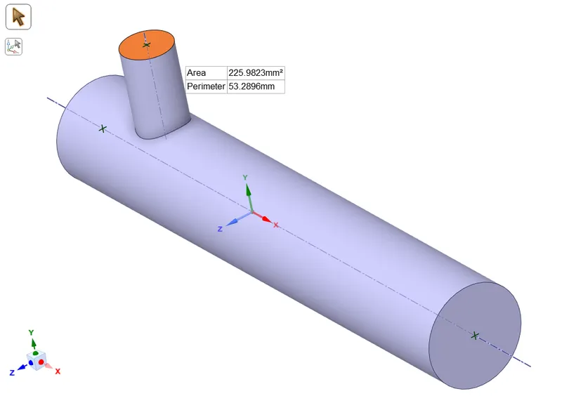
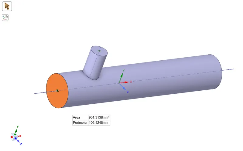
Short Mixing Tee Extracted Volume & Cold inlet area		Short Mixing Tee Extracted Volume & Hot inlet area

Long Mixing Tee Geometry:

Long Mixing Tee Geometry & Cold inlet area		Long Mixing Tee Geometry & Hot inlet area
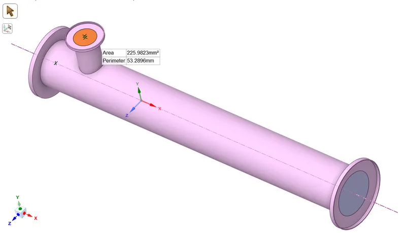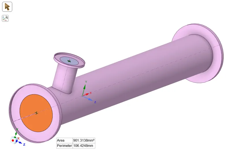Long Mixing Tee Extracted Volume & Cold inlet area		Long Mixing Tee Extracted Volume & Hot inlet area

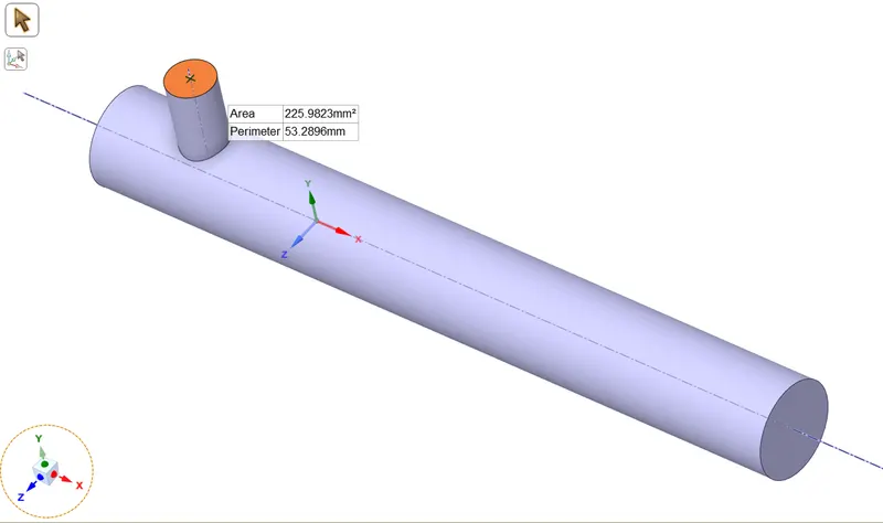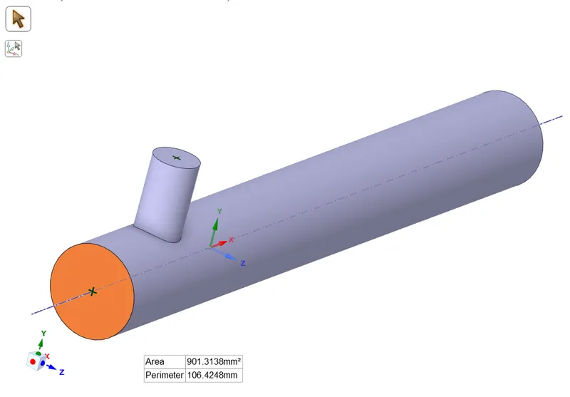(I) Case 1-a  and  Case 1-b with k-epsilon viscous model:

• Short mixing Tee with  `V_h = 3  m/s` `V_(ca) = 6  m/s` and `V_(cb) = 12  m/s`.
• Mesh:
  
  
  
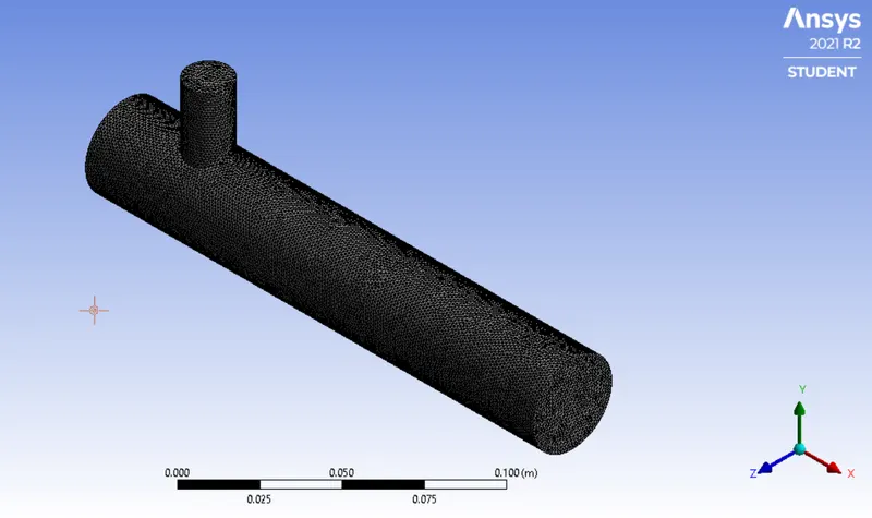
• Mesh Quality and Mesh Metrics:
  
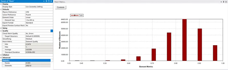
• Energy and turbulance model k- epsilon settings:
  
  
  
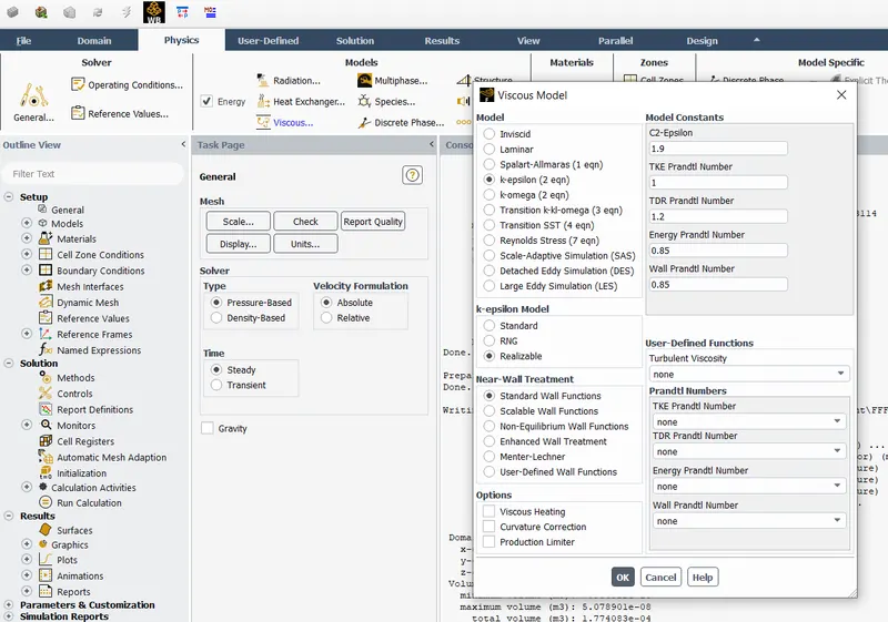
• Material Properties setting 
  
  
  
  
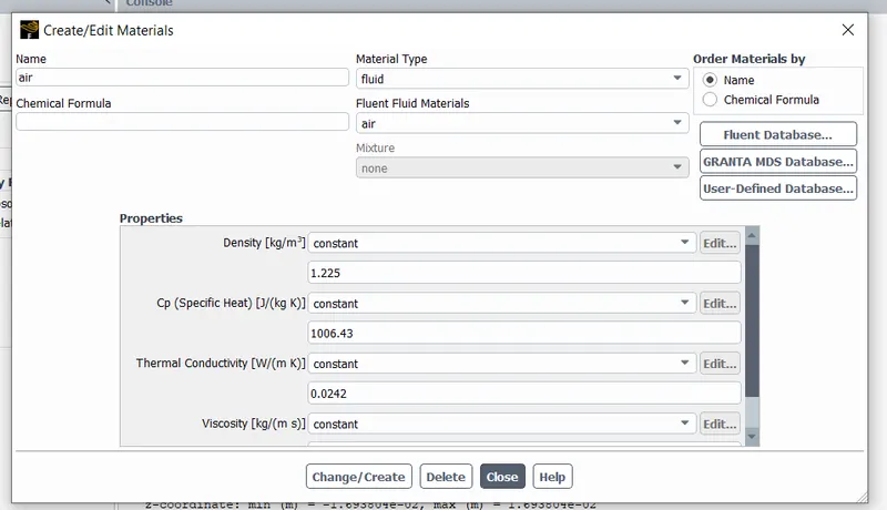
• Cell Zone Condition
  
  
  
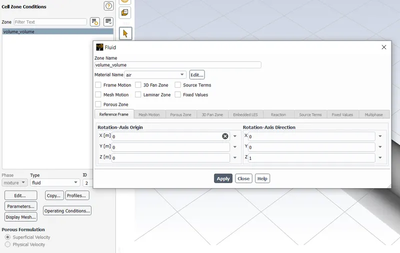
• Boundary Conditions
  

  Case (1-a) - Hot air inlet- Velocity		Case (1-a) - Hot air inlet -Temperature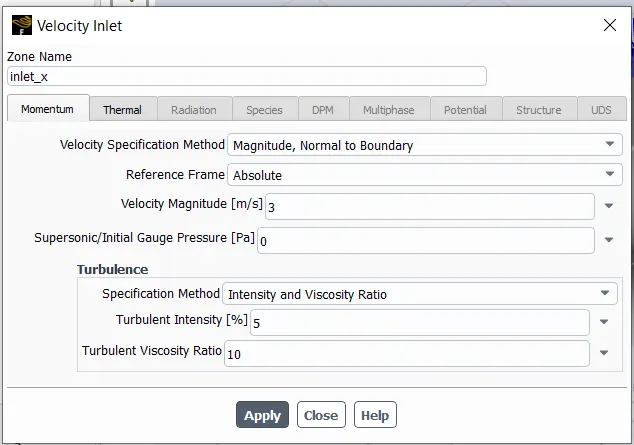
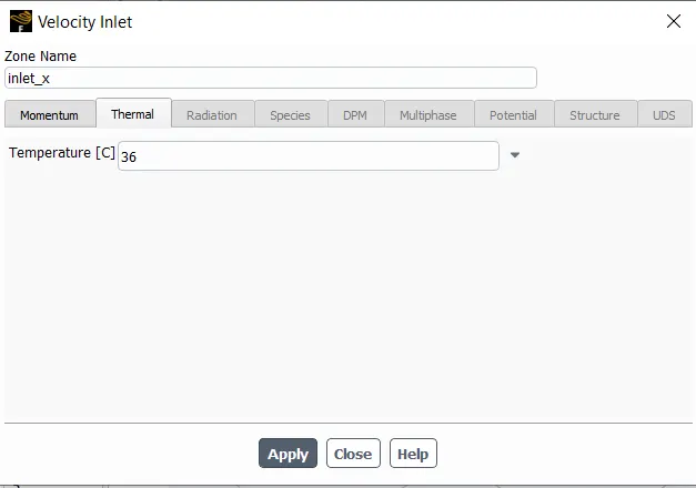
  Case (1-a) - Cold air inlet- Velocity		Case (1-a) - Cold air inlet -Temperature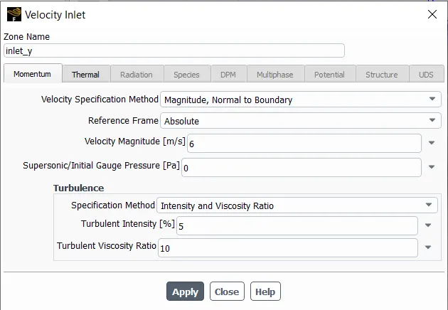
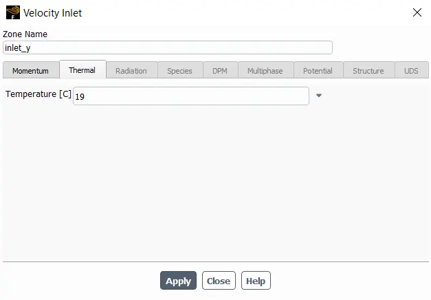
  Case (1-b) - Hot air inlet - Velocity		Case (1-b) - Hot air inlet - Temperature
  Case (1-b) - Cold air inlet - Velocity		Case (1-b) - Cold air inlet - Temperature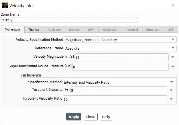

  
  
  
• Reports
  
  

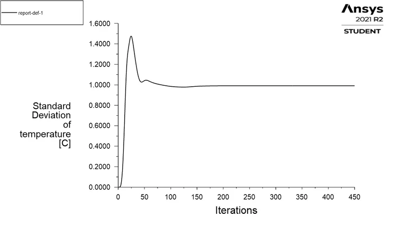
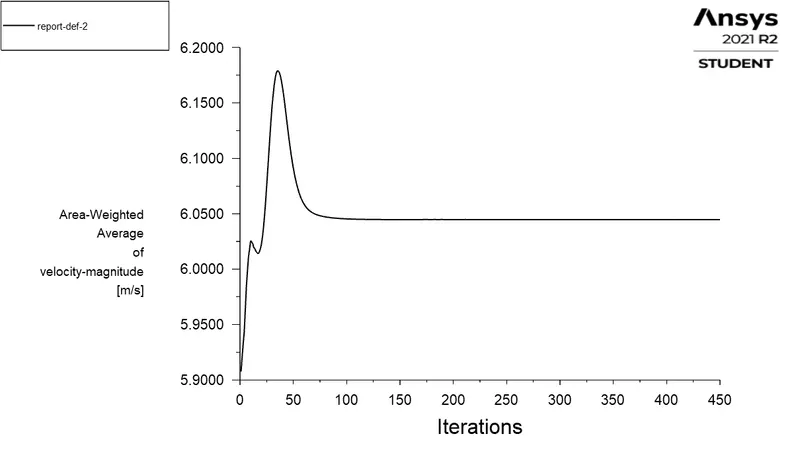
  	Case 1-a (k-epsilon 140 Iterations)			Case 1-b (k-epsilon 450 Iterations)
  1)	Residuals plot (Convergence Plot)		1)	Residuals plot (Convergence Plot)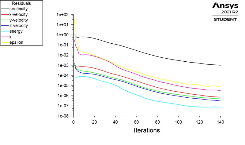
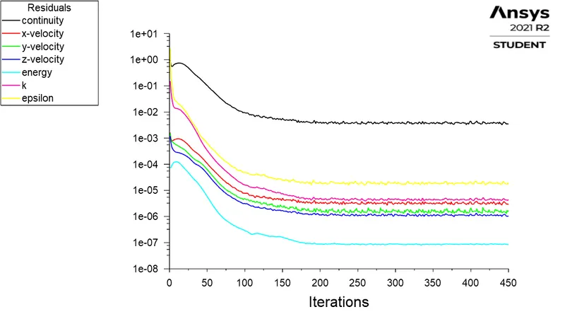
  2)	Area Weighted Average of Outlet Temperature		2)	Area Weighted Average of Outlet Temperature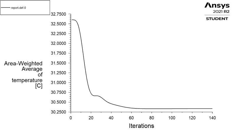
  3)	Standard deviation of Outlet Temperature		3)	Standard deviation of Outlet Temperature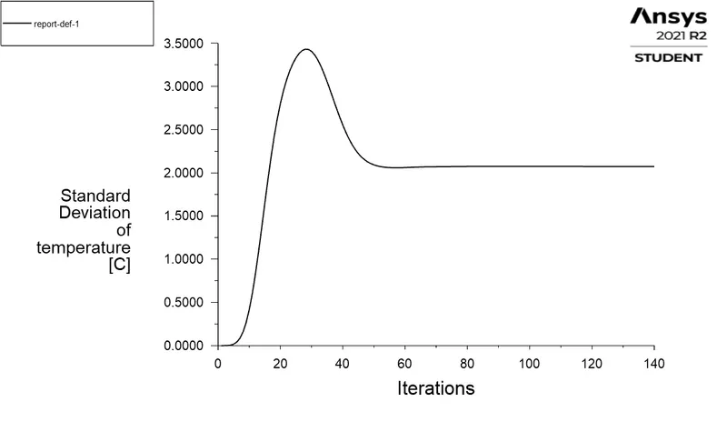
  4)	Area Weighted Average of Outlet Velocity		4)	Area Weighted Average of Outlet Velocity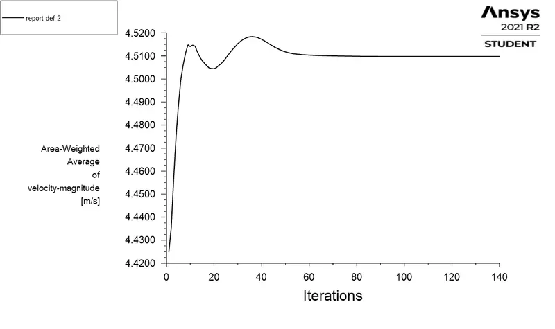

• Results
  
  

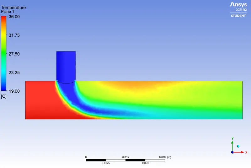
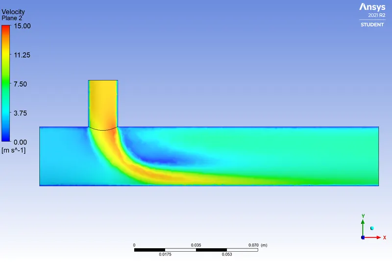
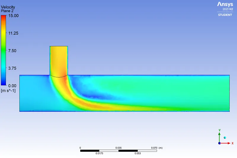
  	Case 1-a (k-epsilon 140 Iterations)			Case 1-b (k-epsilon 450 Iterations)
  1)	Temperature contour (On central plane)		1)	Temperature contour (On central plane)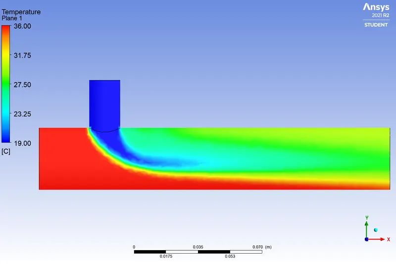
  2)	Velocity contour (On central plane)		2)	Velocity contour (On central plane)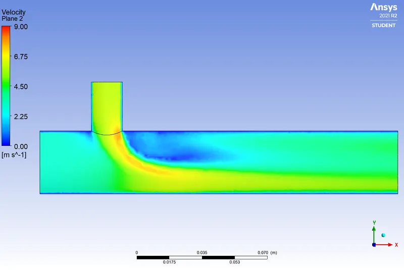
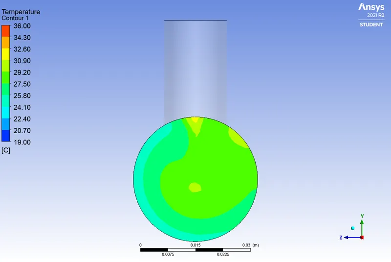
  3)	Temperature contour (On outlet face)		3)	Temperature contour (On outlet face)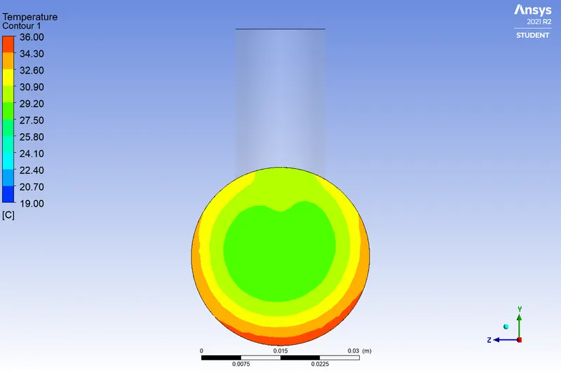
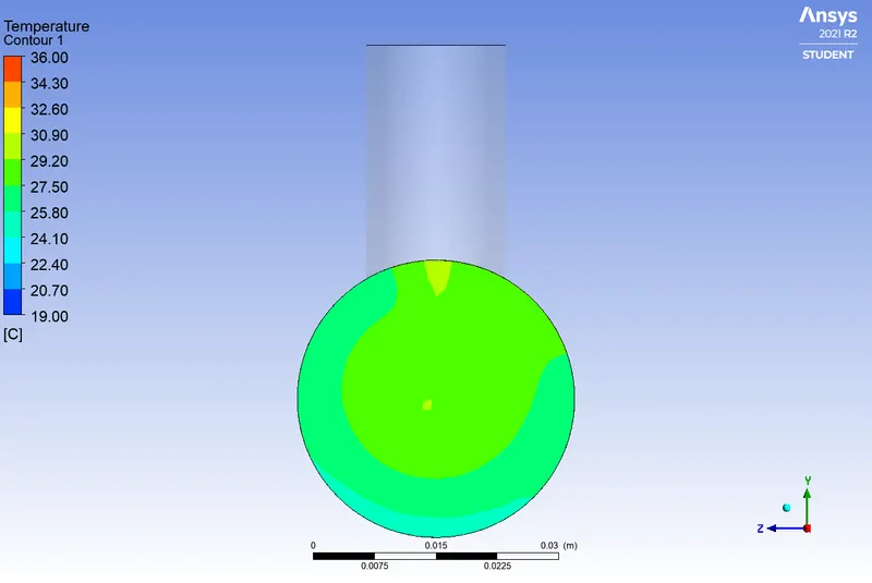
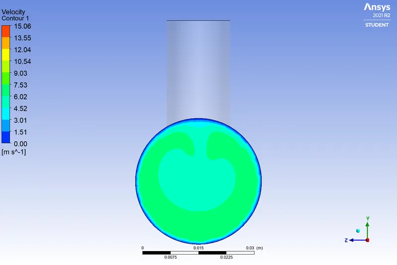
  4)	Velocity contour (On outlet face)		4)	Velocity contour (On outlet face)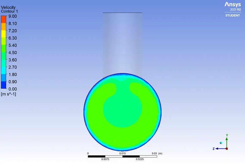
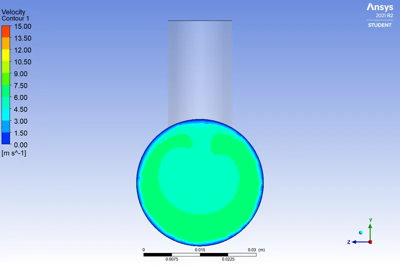
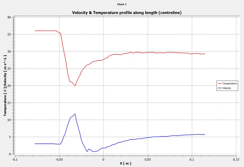
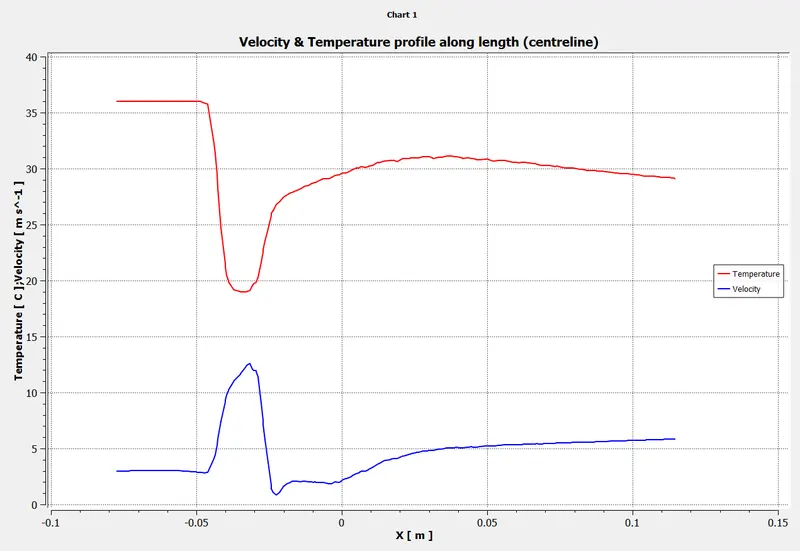
  5)	Velocity & Temperature Plot  (On central line)		5)	Velocity & Temperature Plot  (On central line)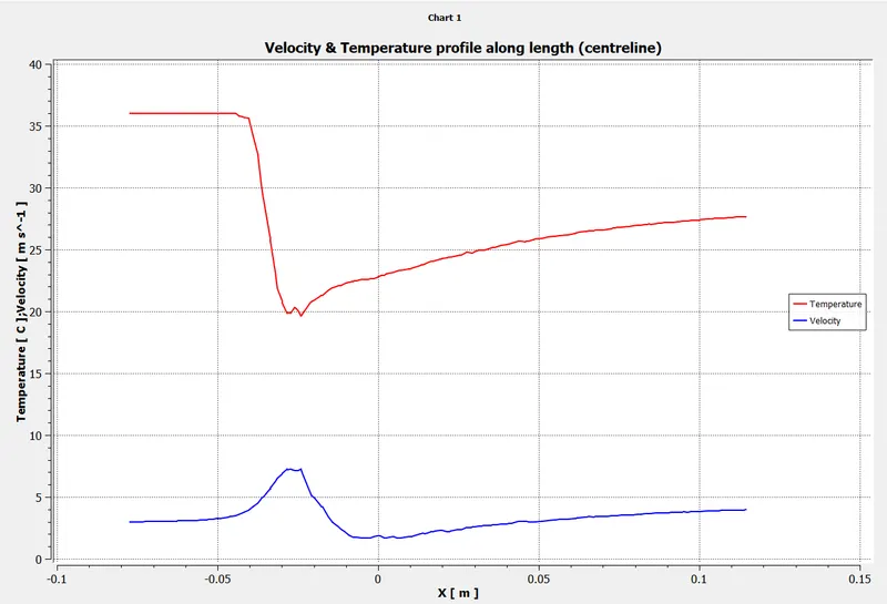

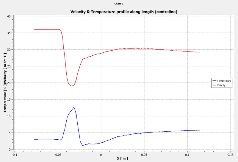
(II) Case 1-a  and  Case 1-b with k-omega viscous model:

• Short mixing Tee with  `V_h = 3  m/s` `V_(ca) = 6  m/s` and `V_(cb) = 12  m/s`.
• Mesh:
  
  
  
• Mesh Quality and Mesh Metrics:
  
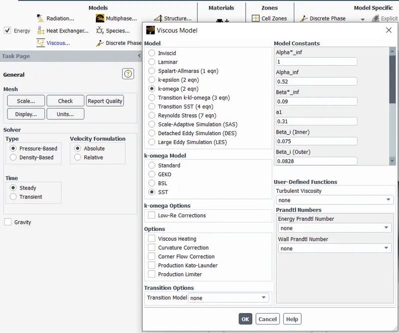
• Energy and turbulance model k - omega settings:
  
  
  
• Material Properties setting 
  
  
  
  
• Cell Zone Condition
  
  
  
• Boundary Conditions
  

  Case (1-a) - Hot air inlet- Velocity		Case (1-a) - Hot air inlet -Temperature
  Case (1-a) - Cold air inlet- Velocity		Case (1-a) - Cold air inlet -Temperature
  Case (1-b) - Hot air inlet - Velocity		Case (1-b) - Hot air inlet - Temperature
  Case (1-b) - Cold air inlet - Velocity		Case (1-b) - Cold air inlet - Temperature

  
  
  
• Reports
  
  

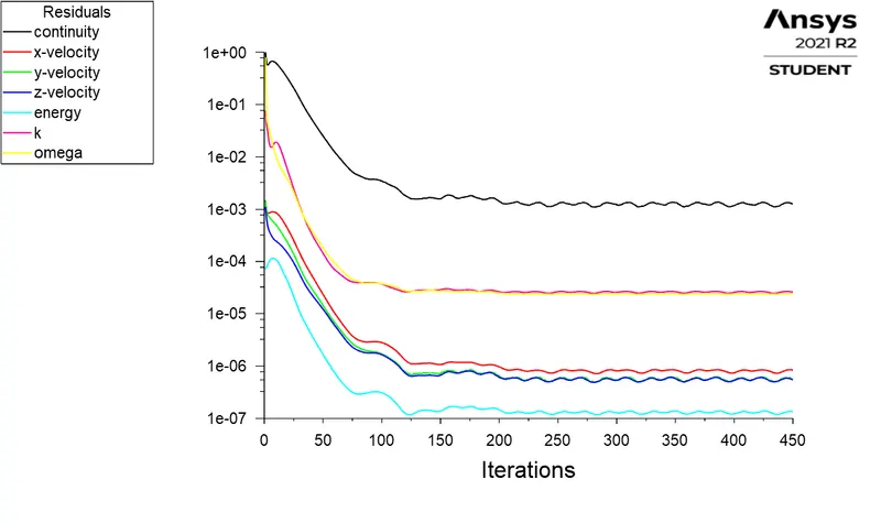
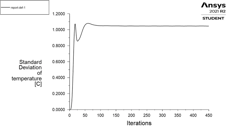
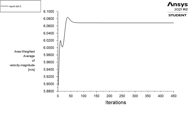
  	Case 1-a (k-omega 114 Iterations)			Case 1-b (k-omega 450 Iterations)
  1)	Residuals plot (Convergence Plot)		1)	Residuals plot (Convergence Plot)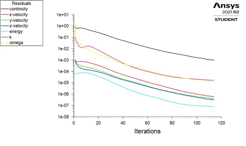
  2)	Area Weighted Average of Outlet Temperature		2)	Area Weighted Average of Outlet Temperature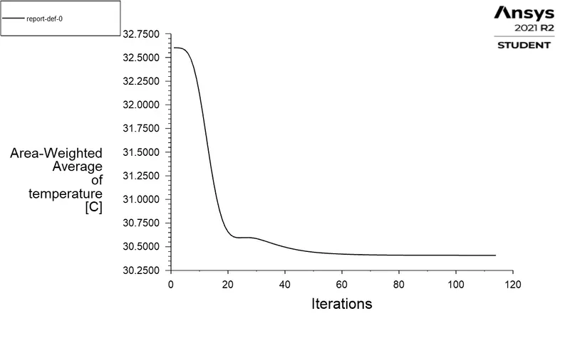
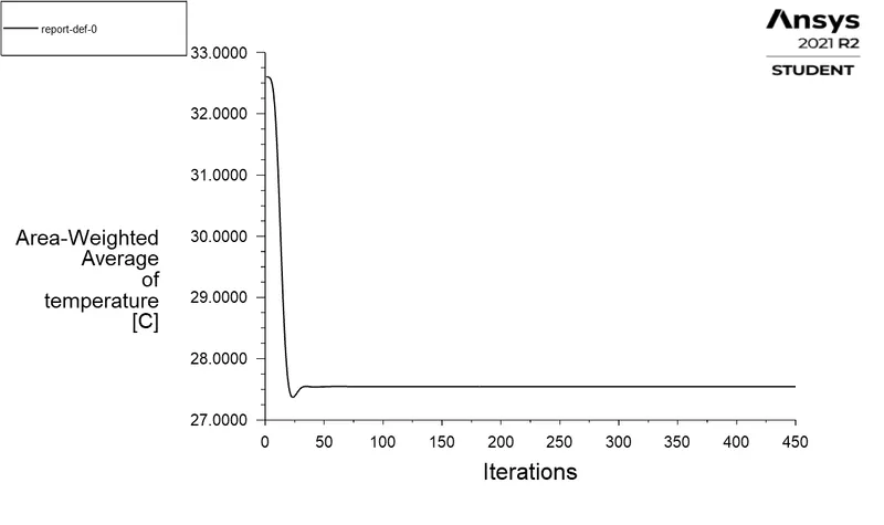
  3)	Standard deviation of Outlet Temperature		3)	Standard deviation of Outlet Temperature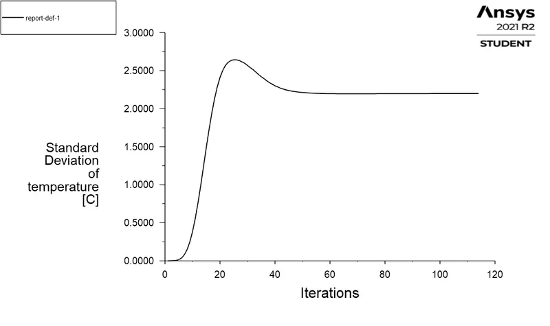
  4)	Area Weighted Average of Outlet Velocity		4)	Area Weighted Average of Outlet Velocity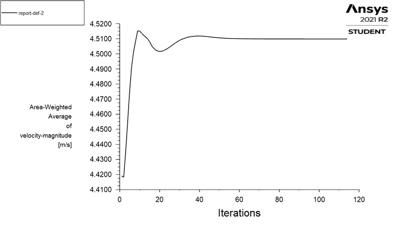

  
  
  
• Results
  
  

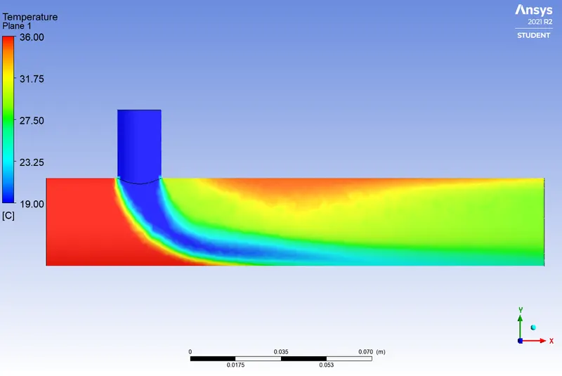
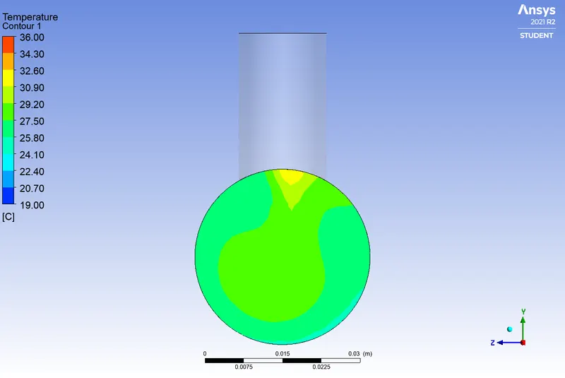
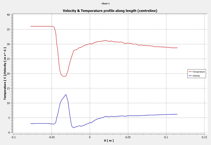
  	Case 1-a (k-omega 114 Iterations)			Case 1-b (k-omega 450 Iterations)
  1)	Temperature contour (On central plane)		1)	Temperature contour (On central plane)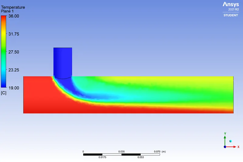
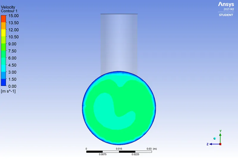
  2)	Velocity contour (On central plane)		2)	Velocity contour (On central plane)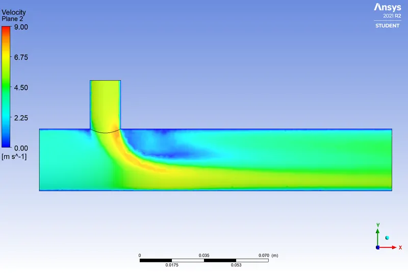
  3)	Temperature contour (On outlet face)		3)	Temperature contour (On outlet face)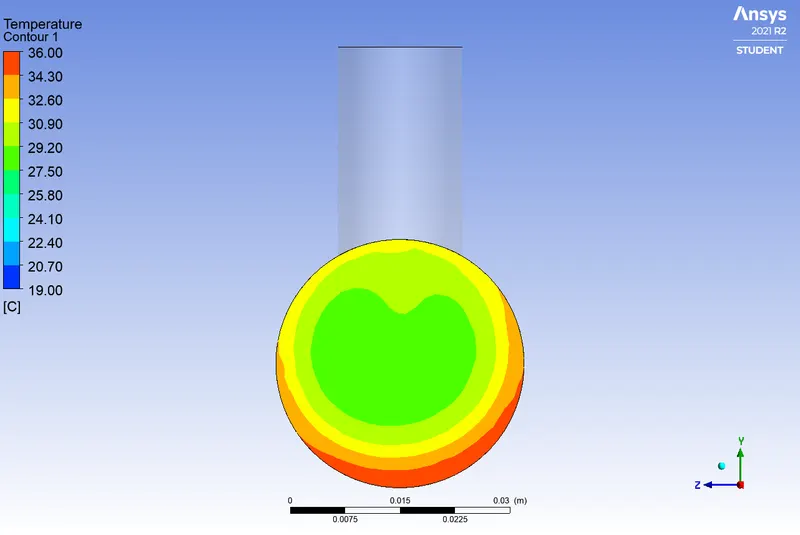
  4)	Velocity contour (On outlet face)		4)	Velocity contour (On outlet face)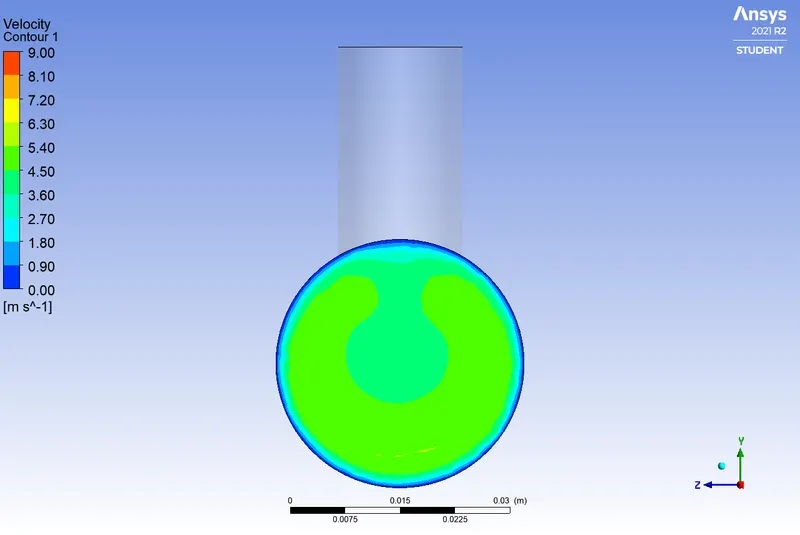
  5)	Velocity & Temperature Plot  (On central line)		5)	Velocity & Temperature Plot  (On central line)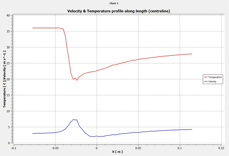

  
  
  
• Table of observation for comparative study between k-epsilon and k-omega SST turbulance models: 
  
  
  
  
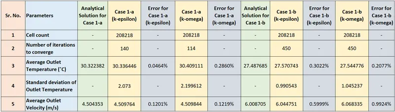
• Generally, k-epsilon turbulance model is used for the free stream simulations and k-omega SST turbulance model is for capturing the phenomenons from the turbulance sublayer. Here our interest is free stream properties thus k-epsilon model is preferred over k-omega SST turbulance model. 
• Also it can be observed from the above comparison table that the results from k-omega SST model have relativeley larger errors and higher standard deviation values for outlet temperature than the results from k-epsilon turbulance models thus k-epsilon turbulance model is considered for further simulations.   

(III) Case 2-a  and  Case 2-b with k-epsilon viscous model:

• Long mixing Tee with  `V_h = 3  m/s` `V_(ca) = 6  m/s` and `V_(cb) = 12  m/s`.
• Mesh:
  
  
  
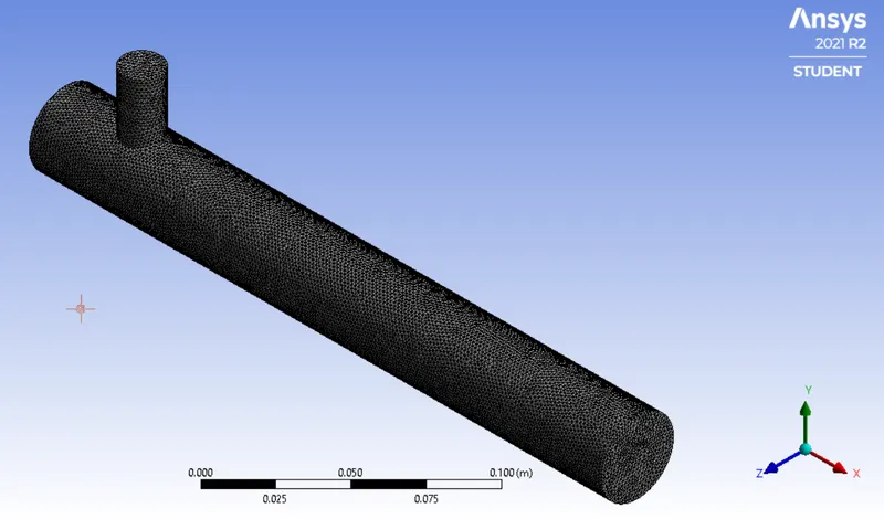
• Mesh Quality and Mesh Metrics:
  
  
  
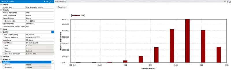
• Energy and turbulance model k- epsilon settings:
  
  
  
• Material Properties setting 
  
  
  
  
• Cell Zone Condition
  
  
  
• Boundary Conditions
  

  Case (2-a) - Hot air inlet- Velocity		Case (2-a) - Hot air inlet -Temperature
  Case (2-a) - Cold air inlet- Velocity		Case (2-a) - Cold air inlet -Temperature
  Case (2-b) - Hot air inlet - Velocity		Case (2-b) - Hot air inlet - Temperature
  Case (2-b) - Cold air inlet - Velocity		Case (2-b) - Cold air inlet - Temperature

  
  
  
• Reports
  
  

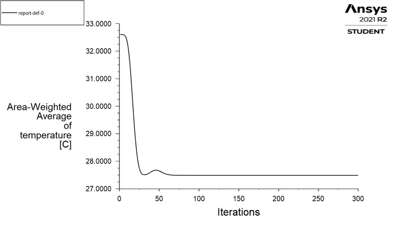
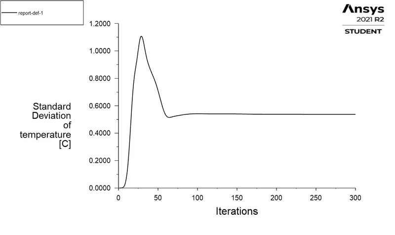
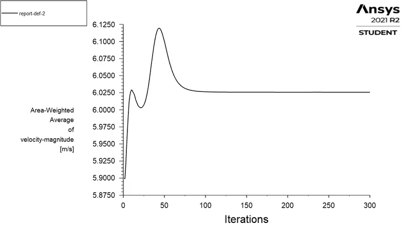
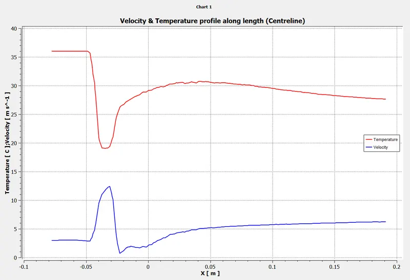
  	Case 2-a (k-epsilon 143 Iterations)			Case 2-b (k-epsilon 300 Iterations)
  1)	Residuals plot (Convergence Plot)		1)	Residuals plot (Convergence Plot)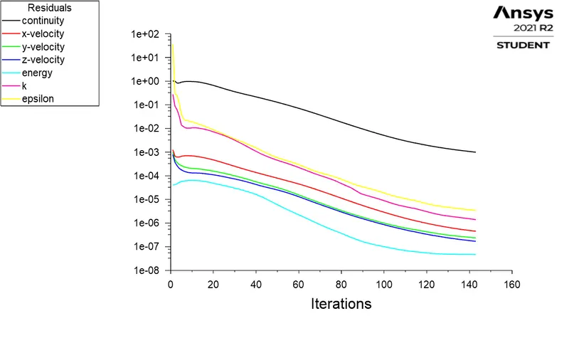
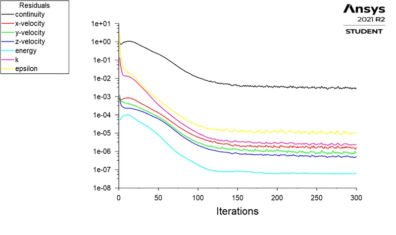
  2)	Area Weighted Average of Outlet Temperature		2)	Area Weighted Average of Outlet Temperature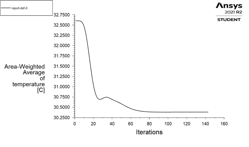
  3)	Standard deviation of Outlet Temperature		3)	Standard deviation of Outlet Temperature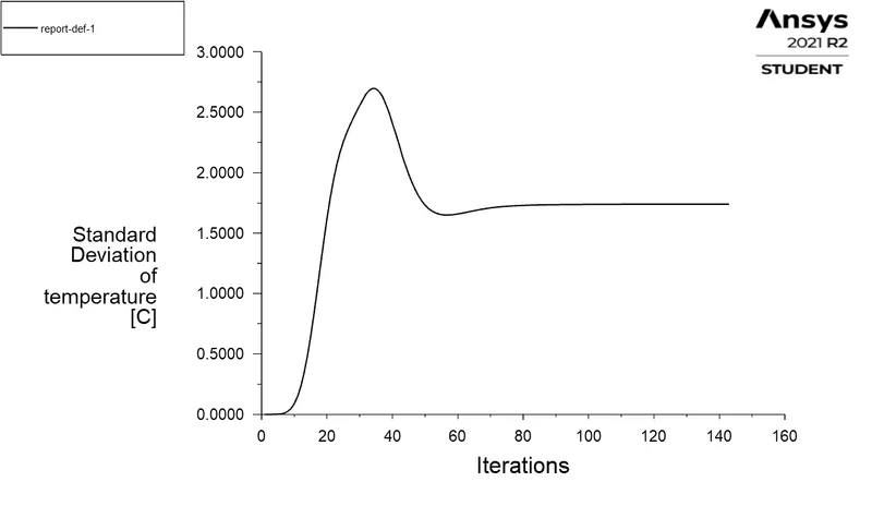
  4)	Area Weighted Average of Outlet Velocity		4)	Area Weighted Average of Outlet Velocity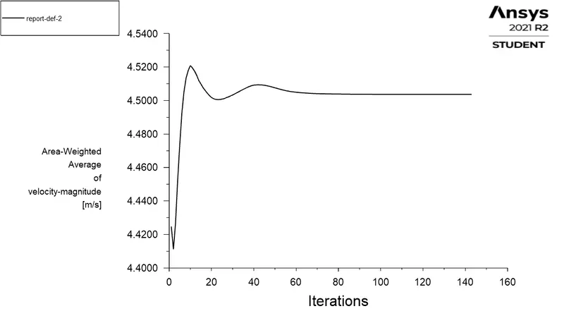

• Results
  
  

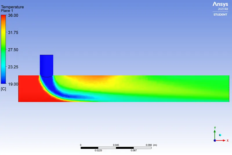
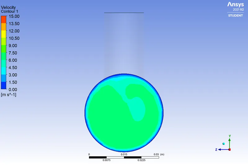
  	Case 2-a (k-epsilon  143 Iterations)			Case 2-b (k-epsilon 300 Iterations)
  1)	Temperature contour (On central plane)		1)	Temperature contour (On central plane)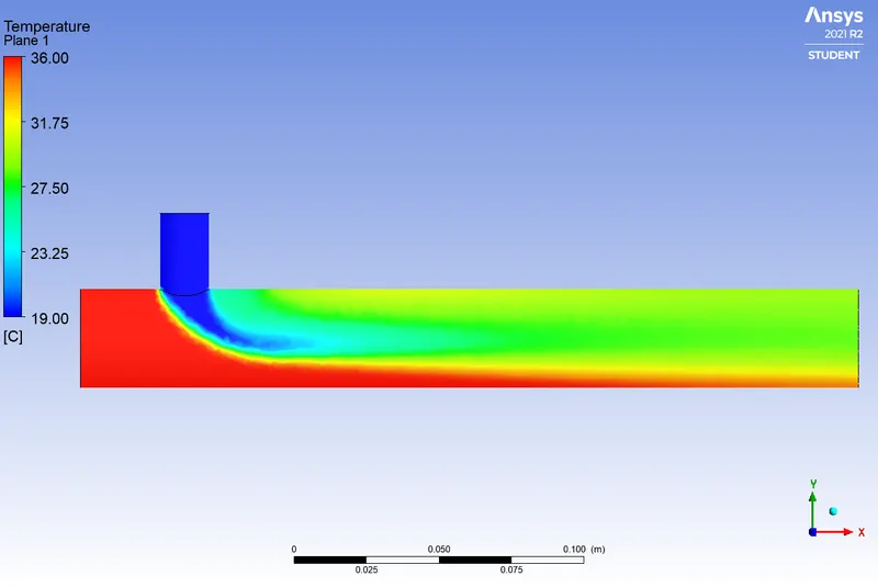
  2)	Velocity contour (On central plane)		2)	Velocity contour (On central plane)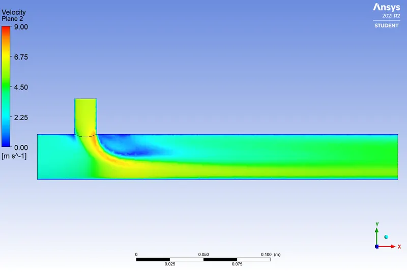
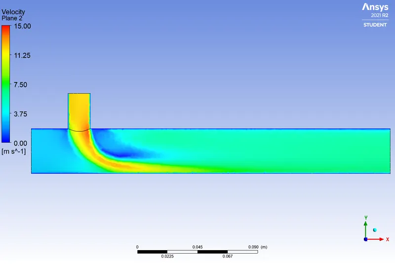
  3)	Temperature contour (On outlet face)		3)	Temperature contour (On outlet face)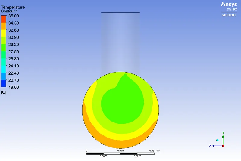
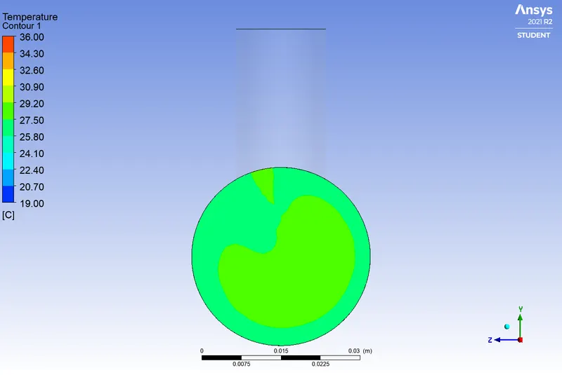
  4)	Velocity contour (On outlet face)		4)	Velocity contour (On outlet face)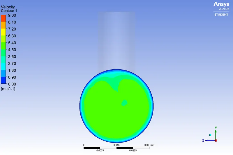
  5)	Velocity & Temperature Plot  (On central line)		5)	Velocity & Temperature Plot  (On central line)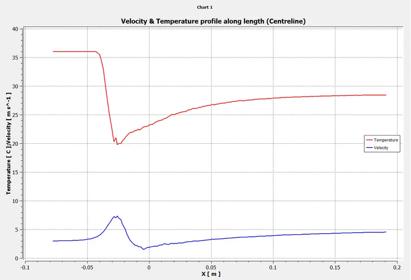

  
  
  
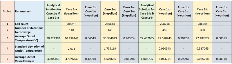
• Table of Observation for Case 1 and Case 2 comparative study (with k epsilon turbulance model):
  
  
  
  

(IV) Case 1-a  and  Case 1-b with k-epsilon viscous model & Coarse Mesh:

• Short mixing Tee with  `V_h = 3  m/s` `V_(ca) = 6  m/s` and `V_(cb) = 12  m/s`.
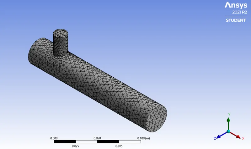
• Mesh:
  
  
  
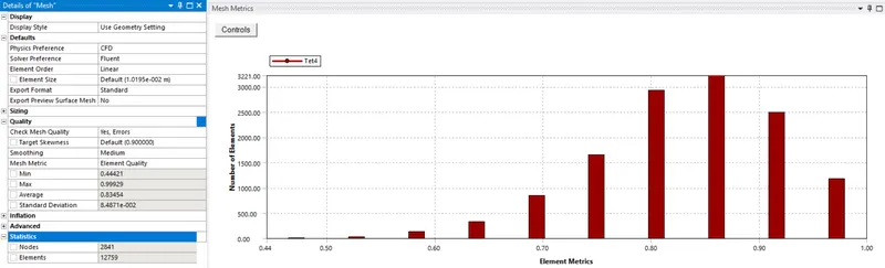
• Mesh Quality and Mesh Metrics:
  
  
  
• Energy and turbulance model k- epsilon settings:
  
  
  
• Material Properties setting 
  
  
  
  
• Cell Zone Condition
  
  
  
• Boundary Conditions
  
  

  Case (1-a) - Hot air inlet- Velocity		Case (1-a) - Hot air inlet -Temperature
  Case (1-a) - Cold air inlet- Velocity		Case (1-a) - Cold air inlet -Temperature
  Case (1-b) - Hot air inlet - Velocity		Case (1-b) - Hot air inlet - Temperature
  Case (1-b) - Cold air inlet - Velocity		Case (1-b) - Cold air inlet - Temperature

  
  
  
• Reports
  
  

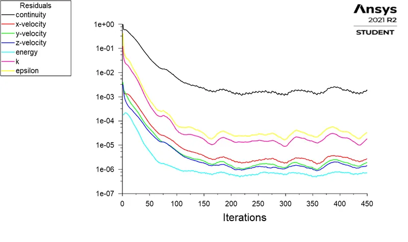
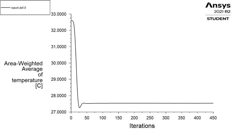
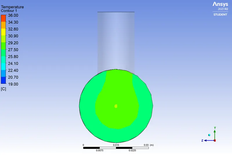
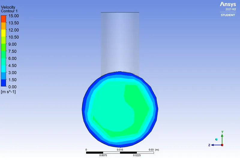
  	Case 1-a (k-epsilon /Coarse Mesh 276 Iterations)			Case 1-b (k-epsilon /Coarse Mesh 450 Iterations)
  1)	Residuals plot (Convergence Plot)		1)	Residuals plot (Convergence Plot)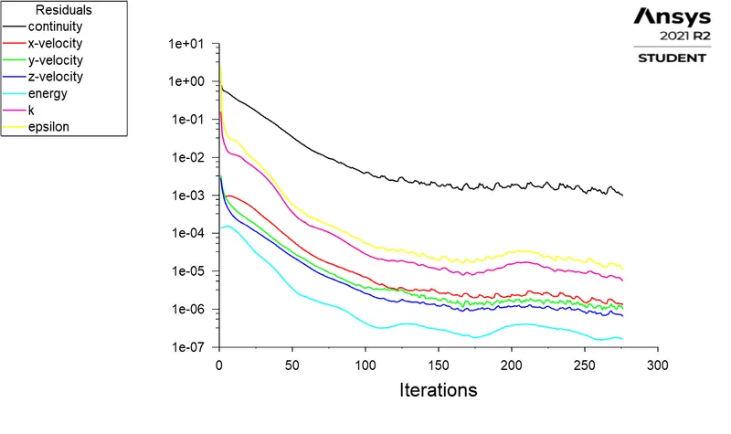
  2)	Area Weighted Average of Outlet Temperature		2)	Area Weighted Average of Outlet Temperature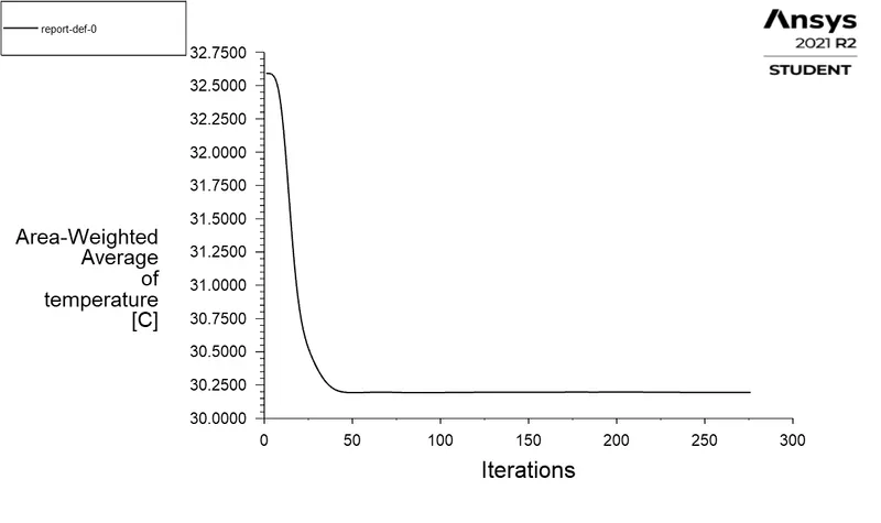
  3)	Standard deviation of Outlet Temperature		3)	Standard deviation of Outlet Temperature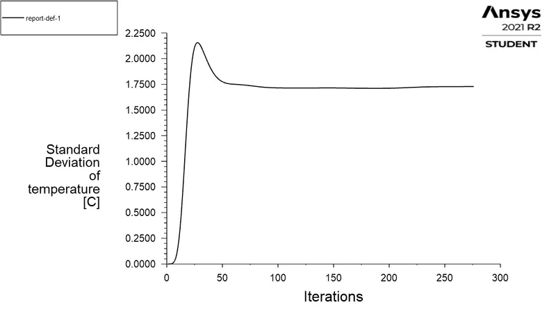
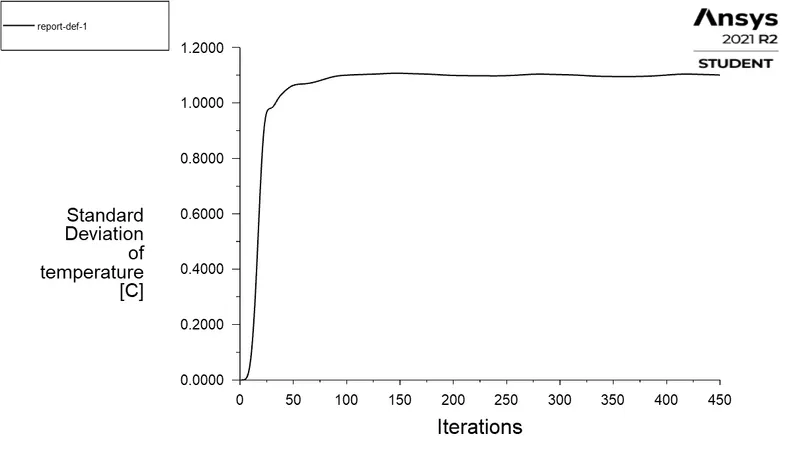
  4)	Area Weighted Average of Outlet Velocity		4)	Area Weighted Average of Outlet Velocity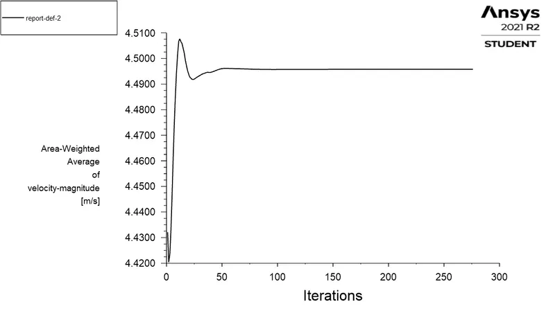

  
  
  
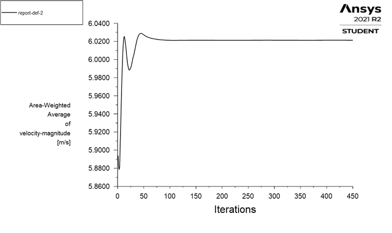
• Results
  
  

  	Case 1-a (k-epsilon  /Coarse Mesh 276 Iterations)			Case 1-b (k-epsilon /Coarse Mesh 450 Iterations)
  1)	Temperature contour (On central plane)		1)	Temperature contour (On central plane)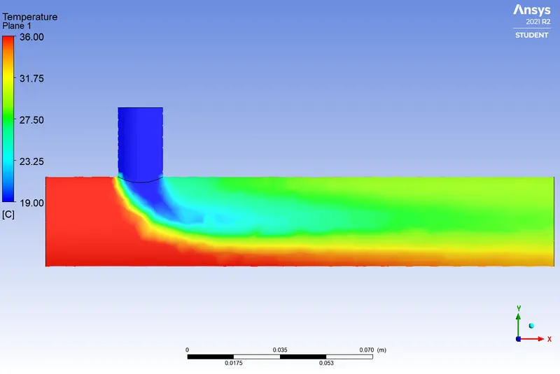
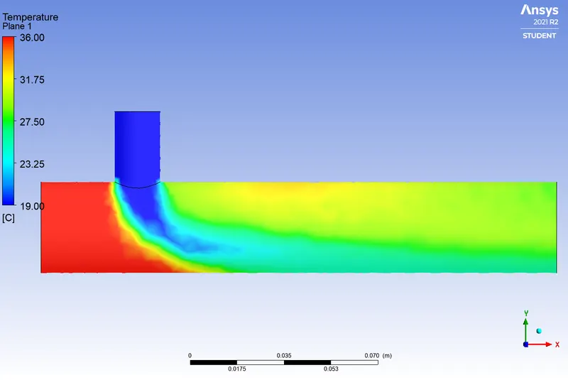
  2)	Velocity contour (On central plane)		2)	Velocity contour (On central plane)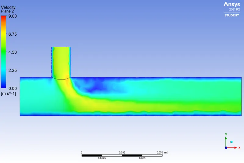
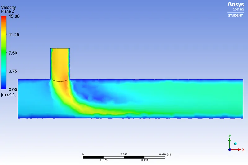
  3)	Temperature contour (On outlet face)		3)	Temperature contour (On outlet face)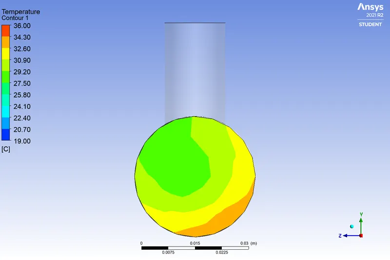
  4)	Velocity contour (On outlet face)		3)	Velocity contour (On outlet face)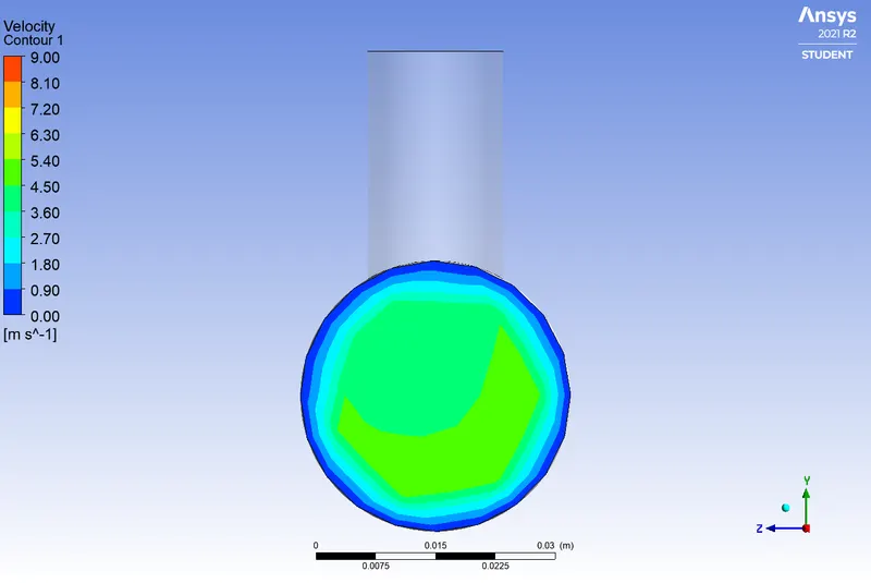
  5)	Velocity & Temperature Plot  (On central line)		4)	Velocity & Temperature Plot  (On central line)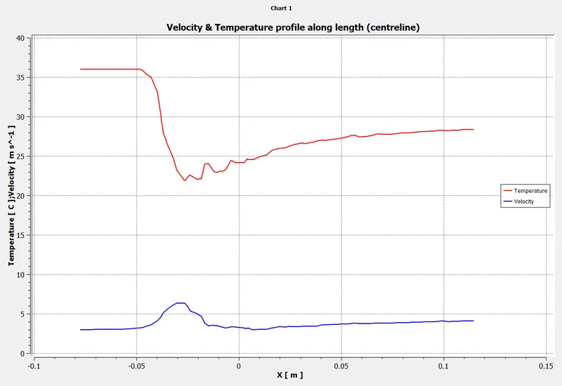

(V) Case 1-a  and  Case 1-b with k-epsilon viscous model & Fine Mesh:

• Short mixing Tee with  `V_h = 3  m/s` `V_(ca) = 6  m/s` and `V_(cb) = 12  m/s`.
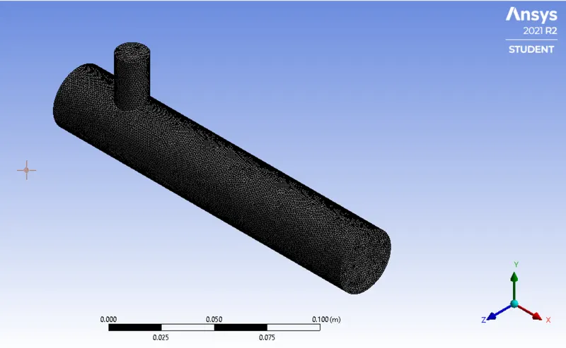
• Mesh:
  
  
  
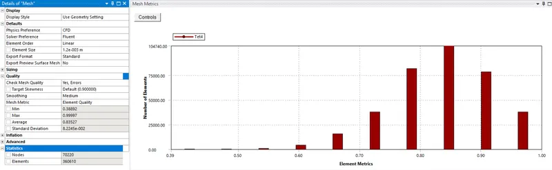
• Mesh Quality and Mesh Metrics:
  
  
  
• Energy and turbulance model k- epsilon settings:
  
  
  
• Material Properties setting 
  
  
  
  
• Cell Zone Condition
  
  
  
• Boundary Conditions
  

  Case (1-a) - Hot air inlet- Velocity		Case (1-a) - Hot air inlet -Temperature
  Case (1-a) - Cold air inlet- Velocity		Case (1-a) - Cold air inlet -Temperature
  Case (1-b) - Hot air inlet - Velocity		Case (1-b) - Hot air inlet - Temperature
  Case (1-b) - Cold air inlet - Velocity		Case (1-b) - Cold air inlet - Temperature

  
  
  
• Reports
  
  

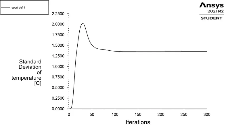
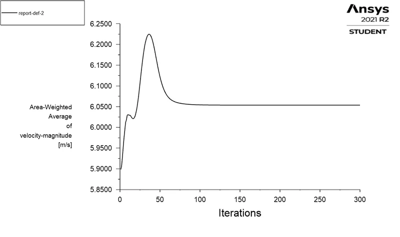
  	Case 1-a (k-epsilon /Fine Mesh 126 Iterations)			Case 1-b (k-epsilon /Fine Mesh 300 Iterations)
  1)	Residuals plot (Convergence Plot)		1)	Residuals plot (Convergence Plot)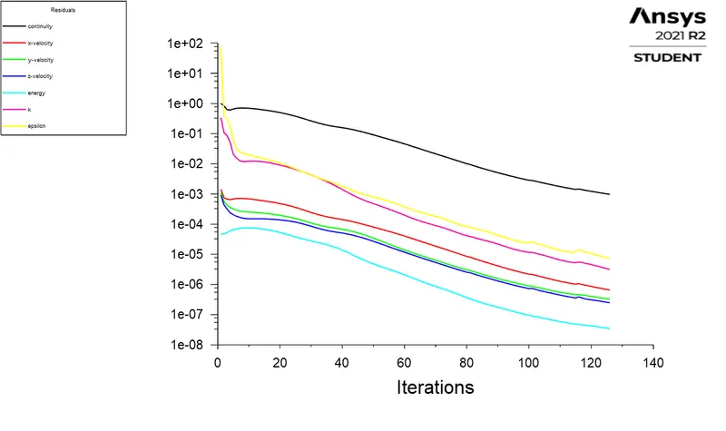
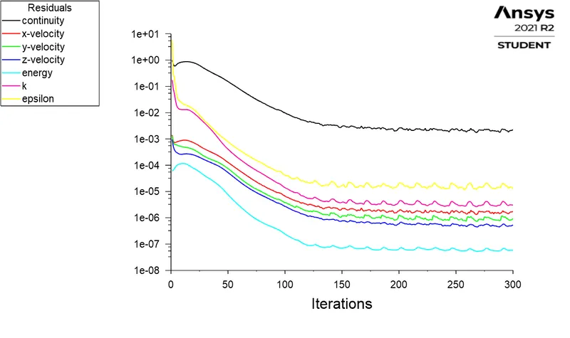
  2)	Area Weighted Average of Outlet Temperature		2)	Area Weighted Average of Outlet Temperature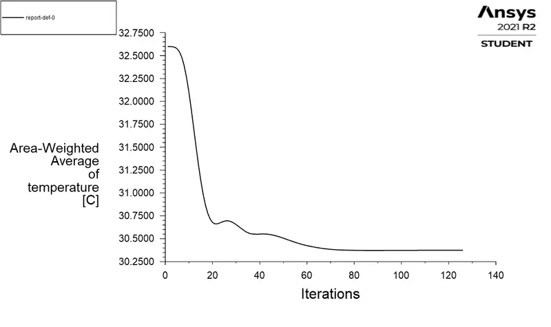
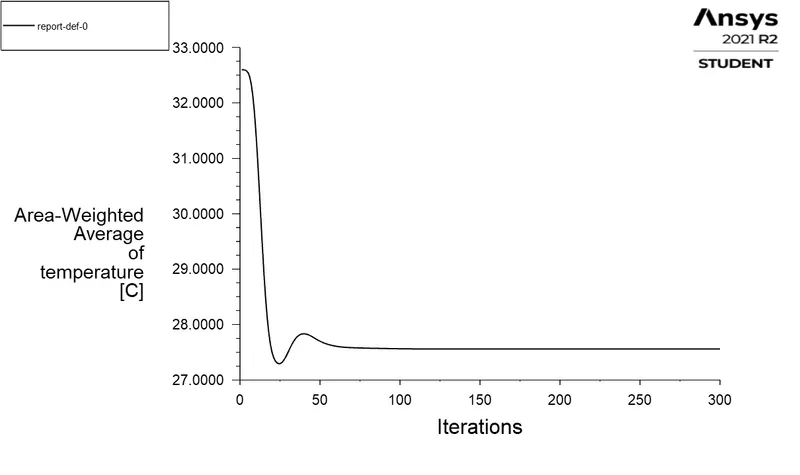
  3)	Standard deviation of Outlet Temperature		3)	Standard deviation of Outlet Temperature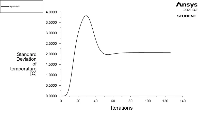
  4)	Area Weighted Average of Outlet Velocity		4)	Area Weighted Average of Outlet Velocity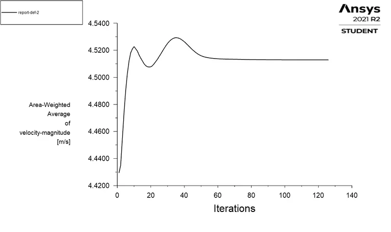

• Results
  
  

  	Case 1-a (k-epsilon  /Fine Mesh 126 Iterations)			Case 1-b (k-epsilon /Fine Mesh 300 Iterations)
  1)	Temperature contour (On central plane)		1)	Temperature contour (On central plane)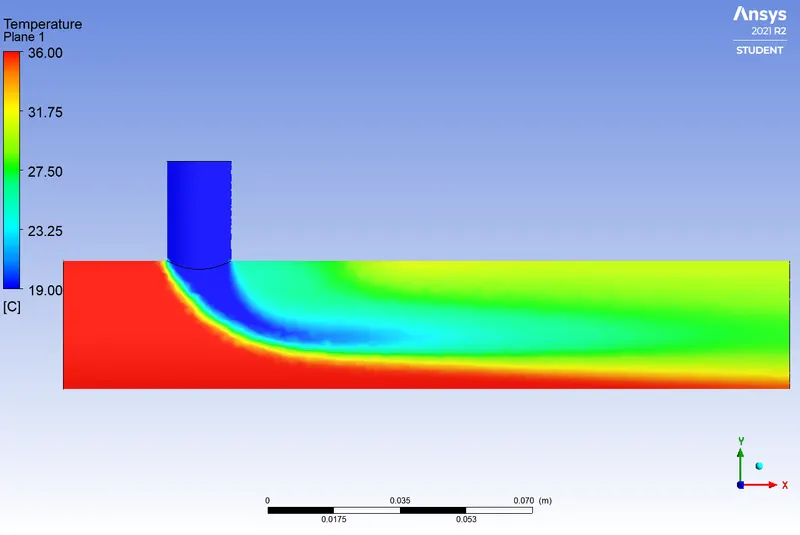
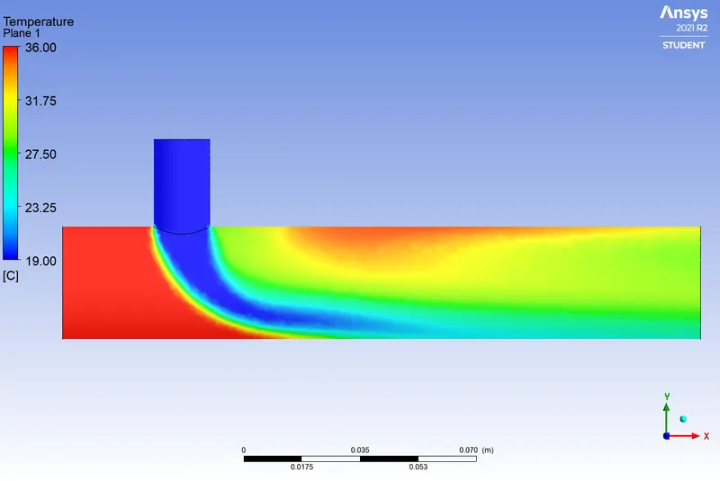
  2)	Velocity contour (On central plane)		2)	Velocity contour (On central plane)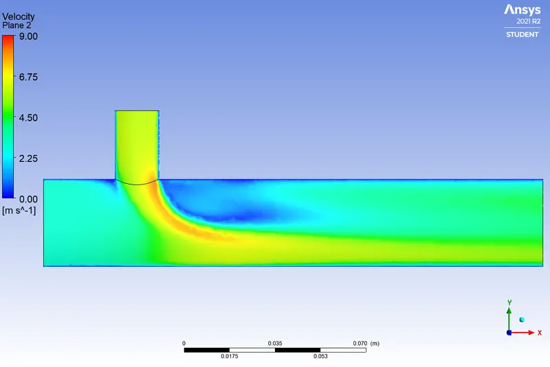
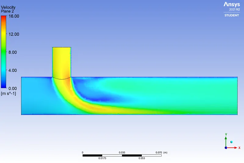
  3)	Temperature contour (On outlet face)		3)	Temperature contour (On outlet face)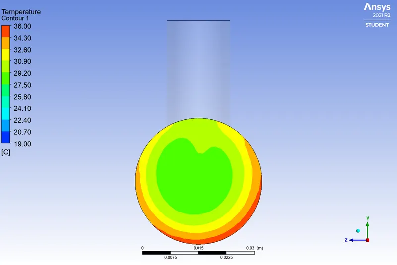
  4)	Velocity contour (On outlet face)		4)	Velocity contour (On outlet face)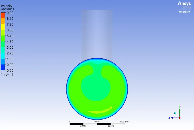
  5)	Velocity & Temperature Plot  (On central line)		5)	Velocity & Temperature Plot  (On central line)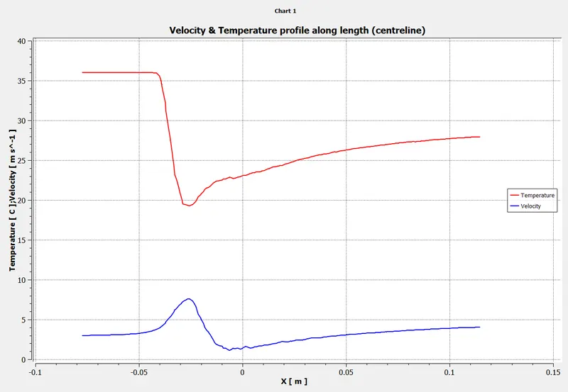

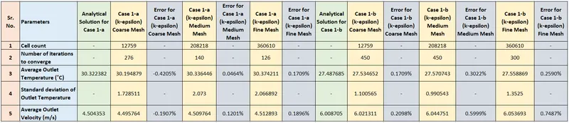
• Table of Observation for Mesh Independance (Grid Independance) study:
  
  
  
  

 Observations & Conclusions:

1. From the comparative study of the k-epsilon and k-omega SST turbulance models, here k-epsilon model is more suitable as these simulations doesnot involve boundary layer or surface phenomenons for the study.
2. From the comparative study of Case 1 and Case 2, it can be observed that the length of the mixing tee has no impact on the average outlet temperature though the less standard deviation of outlet temperature for longer tee shows more uniformality of the temperature over the cross section which is mainly due to diffusion. This can also be observed from the temperature contours on the outlet face.
3. The cold stream velocity has the impact on the outlet temperature. When the cold stream velocity increased while keeping hot stream velocity constant for the respective cold and hot stream temperatures, the outlet temperature decreases significantly.
4. From the table of observation for Mesh independance study, it is can be observed that the results changed significantly as the number of elements increased from 12759 to 208218. But the results have not changed significanlty as number of elements increased further from 208218 to 360610. This indicates that the results are mesh independent. Thus grid convergence is obtained.
5. From above simulations and comparative study the short tee with momentum ratio 4 is better choice if only average outlet temperatue is the main criterion for selection. If uniform temperature distribution over the cross section is major criterion then long tee with momentum ratio is the better choice. This can be observes from temperature contours also.