Mixing Tee analysis for mixing efficiency and different momentum ratios by using K-epsilon and K-omega models.

Mixing TEE CFD simulation

INTRODUCTION

Mixing Tee is a junction device that is having an application for turbulent and temperature mixing. Mixing is performed to allow heat and/or mass transfer to occur between one or more streams, components, or phases. Mixing Tees utilizes a specifically engineered internal geometry to efficiently mix two fluid streams into one combined stream. Mixing tees are widely used in the petrochemical, HVAC industry, etc. in which two fluid streams with different physical and/or chemical properties mix together.

Using different momentum ratios the mixing efficiency is modified.

AIM: CFD analysis to study the mixing efficiency of a Tee joint using ANSYS Fluent using the different turbulent models.

The computational geometry is modeled using URANS based solver namely k-epsilon and k-omega model. With different momentum ratios, physical parameters like no of iterations, cell count, area-weighted average, the standard deviation of temperature at the outlet is predicted. Finally, with different grading of mesh size a grid independence test is conducted to justify the effectiveness of mixing fluids and to measure out the best model for the problem.

OBJECTIVE

• Set up steady-state simulations to compare the mixing effectiveness when hot inlet temperature is 36⁰C & Cold inlet is at 19⁰C.
• Run simulation for long-tee and short-tee geometry based on the RANS model.
• Compare the results based on cell count, number of iterations and outlet temperature of two pipes.
• Perform grid dependence study on any one case.
• Plot thermal and velocity profiles for both geometries.

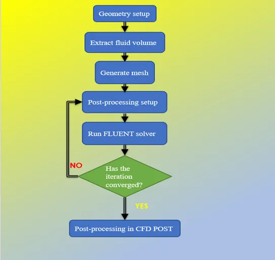
The proper flow chart is shown in the figure below:

TURBULENCE MODELING

K-epsilon Model:

This model is essentially a high Reynolds number model, meaning the law of the wall must be employed and provide velocity “boundary conditions” away from solid boundaries (what is termed “wall-functions”). Another major drawback is the model's lack of sensitivity to adverse pressure-gradient. It was observed that under such conditions it overestimates the shear stress and by that delays separation.

This model is usually used where flow does not demand to integrate the solution through the viscous sublayer and wall-bounded effects are secondary. For such cases, the first cell away from the wall shall be placed at a y+ of 30-300. In such a scenario, the viscous sublayer and buffer layer (viscosity-affected inner region) are not resolved.

Instead, semi-empirical formulas called “wall functions” are used to bridge the viscosity-affected region between the wall and the fully-turbulent region.

K-omega Model:

This model is essentially a low Reynolds number model. This model takes 'elliptic' near-wall behavior meaning that it has an inherent nature of being able to “communicate” with the wall and actually has Dirichlet (as in no-slip in this case) boundary conditions. The implication of such behavior is the straightforward possibility of integrating through the laminar sublayer without additional numerically destabilizing damping functions or two additional transport equations. Commonly encountered situations where the flow demands integrating through the viscous sublayer include: heat transfer, calculation of aerodynamic drag, flows with adverse pressure gradients, etc. Integrating through the viscous sublayer would generally impose resolving the mesh to y+<1. The omega equation can be integrated through the viscous sublayer without the need for a two-layer approach.

1) Pre-Processing

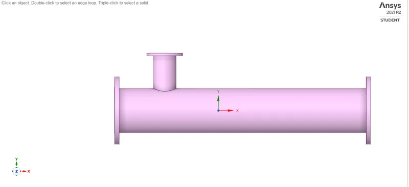
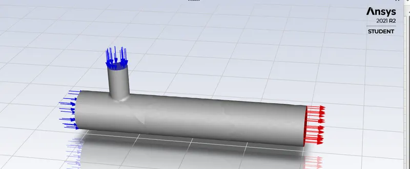
Geometry given is the pipe geometry that cannot be used for analysis. It will be useful when we want results for FSI, heat transfer analysis through walls. Thus we only need fluid volume for analysis.

Fluid volume can be extracted from the feature present in ANSYS Spaceclaim.

Given Geometry

Extracted Fluid Volume

2) Mesh Generation

• The fluid body is opened in Ansys meshing where a default mesh of 10mm is used.
• named selections are created to define all the boundaries inlet-x and inlet-y, outlet, walls for convenience in assigning boundary conditions.
• Mesh is used with wall treatment with inflation layers.
• Click on Update to generate mesh
• A mesh convergence study is carried out for 3 sizes 10mm,5mm and 3mm.

Mesh Size=10mm

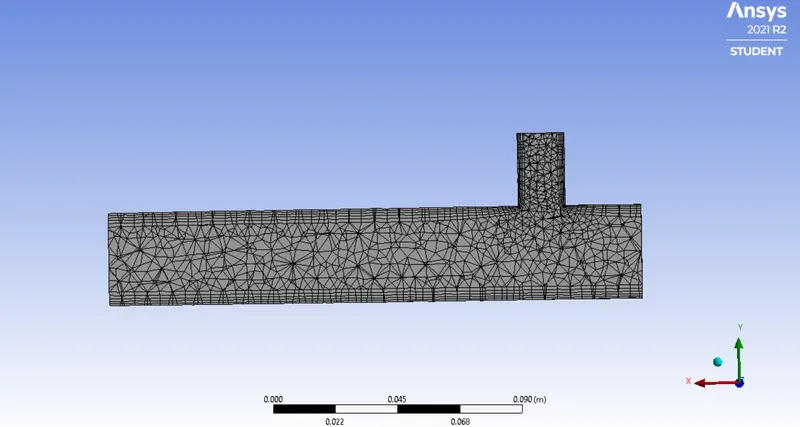
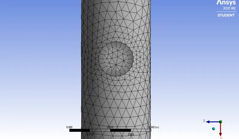
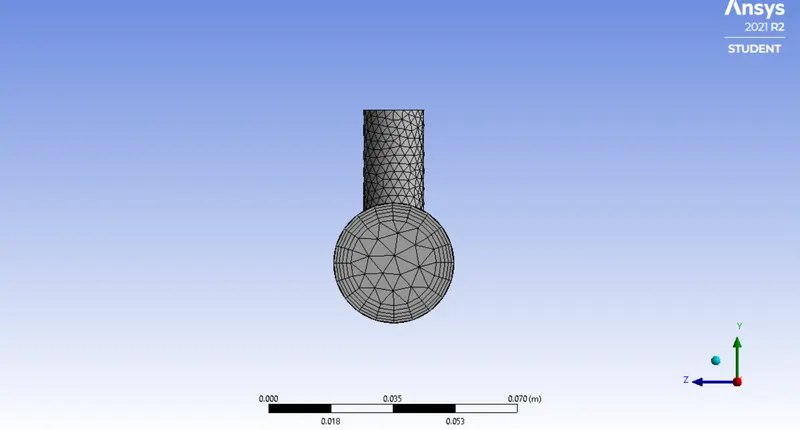
Mesh Size=3mm

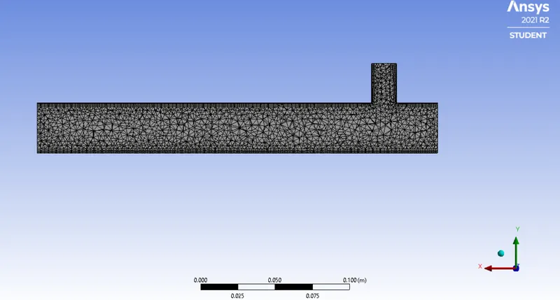
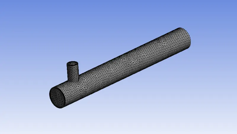
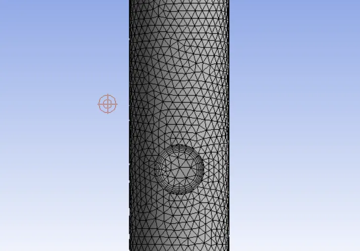
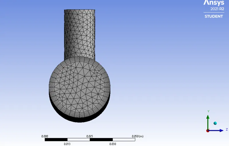
3) Physics Setup

• The FLUENT solver setting is activated, where the console and the graphics pane appear.
• From the General tab, we select the pressure-based solver having absolute velocity formation and within a steady-state condition.
• The energy parameter is activated.
• Then the viscous model is selected, which is k-epsilon Realizable or K-omega SST.
• Specify the material as air.
• Define the boundary condition for inlet x, inlet y, wall by specifying the inlet temperature and velocity.
• Velocity and temperature are assigned as inlet-x velocity as 3m/s and temperature=36C and inlet-y velocity is assigned as per the momentum ratio of 2 or 4 and temperature=19C.
• Initialize the solver with hybrid schemes.
• Set up the no of iterations.
• Click on calculate option.

4) Post Processing Results

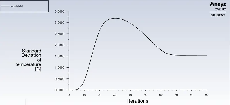
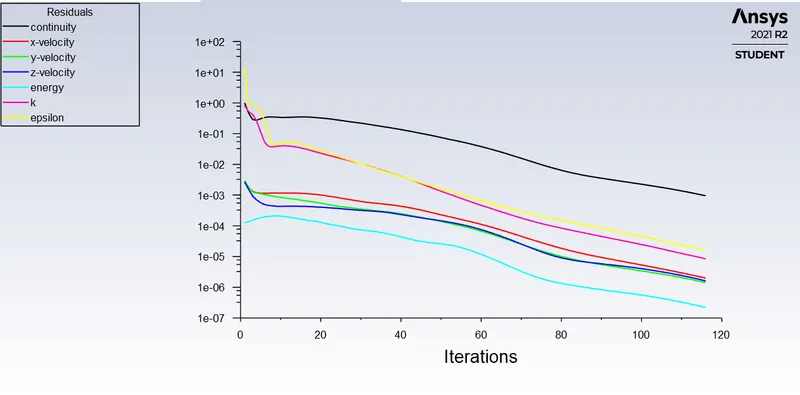
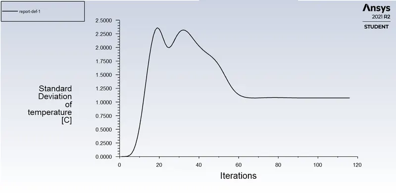
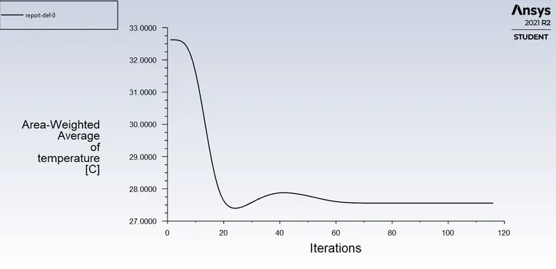
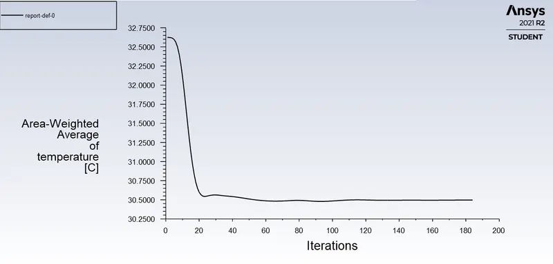
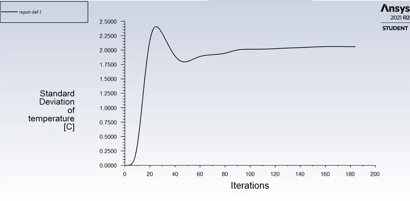
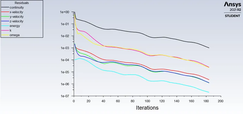
After convergence residuals values, Standard deviation temperature at the outlet, Area weighted average temperature at the outlet is checked.

Open CFD POST and checkmark the inlet, outlet and wall section to view the geometry.

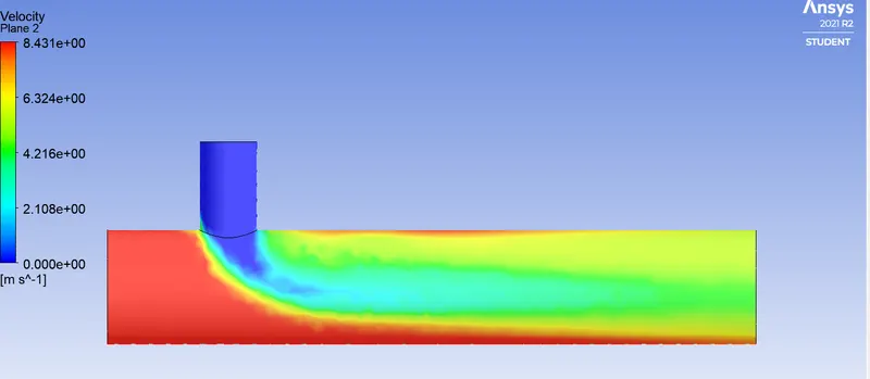
Select planes along and across the geometry of pipe at different crosssections.

Highlight the planes with velocity and temperature variables.

Use line plot along and across the pipe and measure the temperature and velocity variation in a chart.

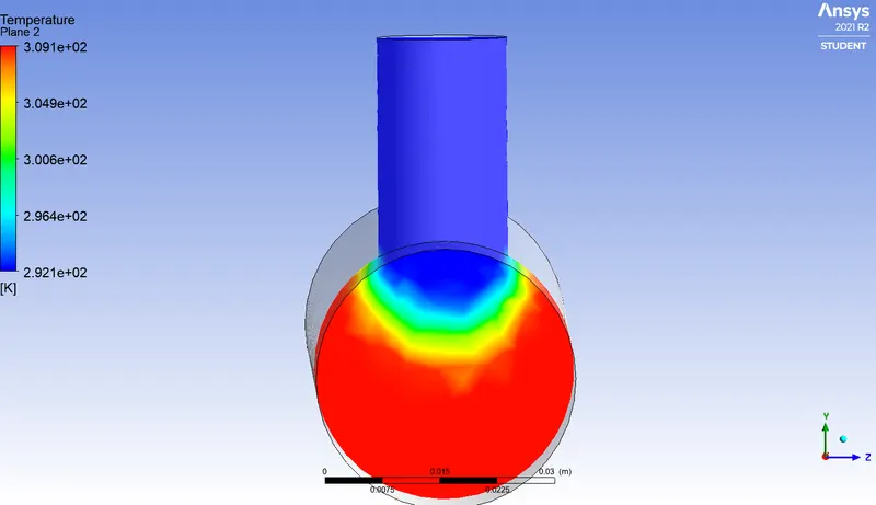
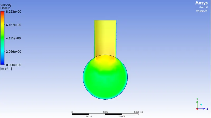
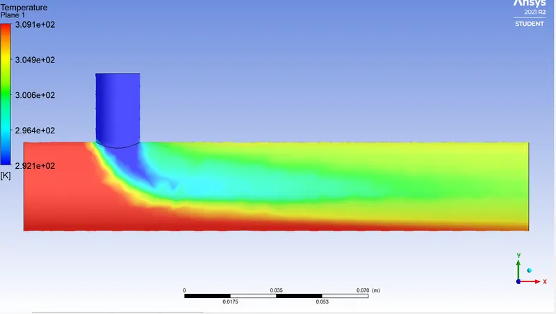
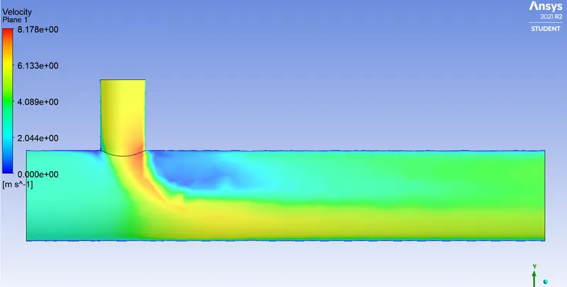
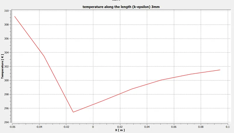
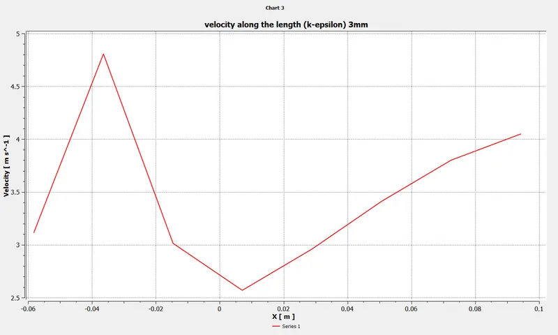
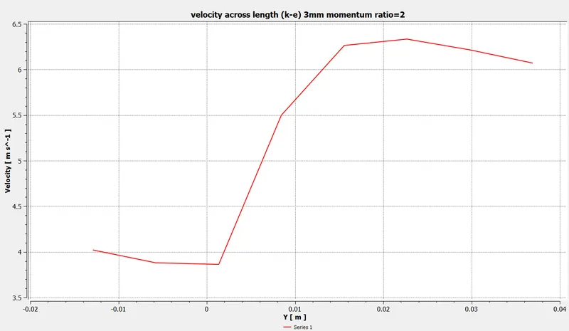
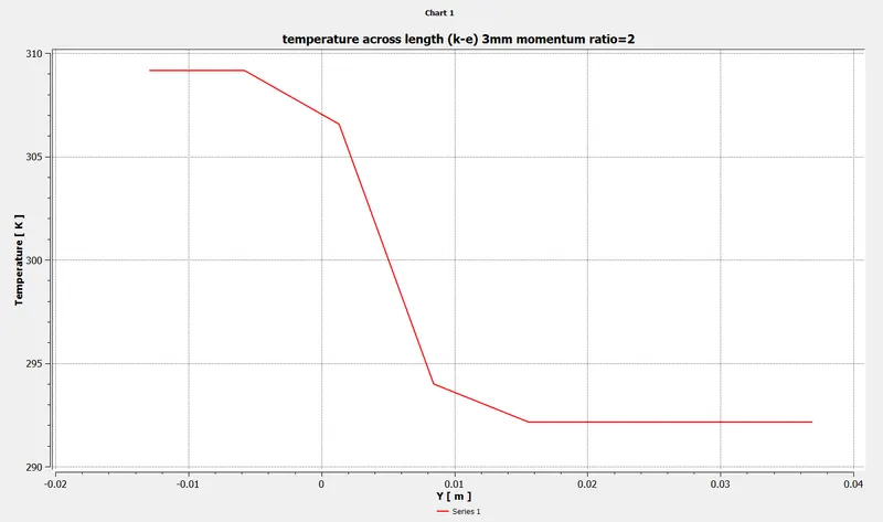
RESULTS for 3mm mesh short pipe momentum ratio=2 with k-epsilon model are shown below:

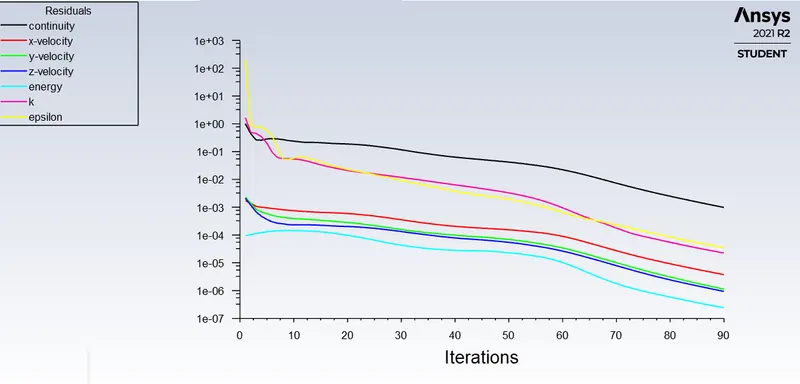
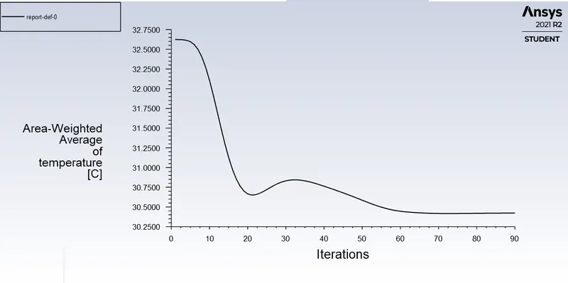
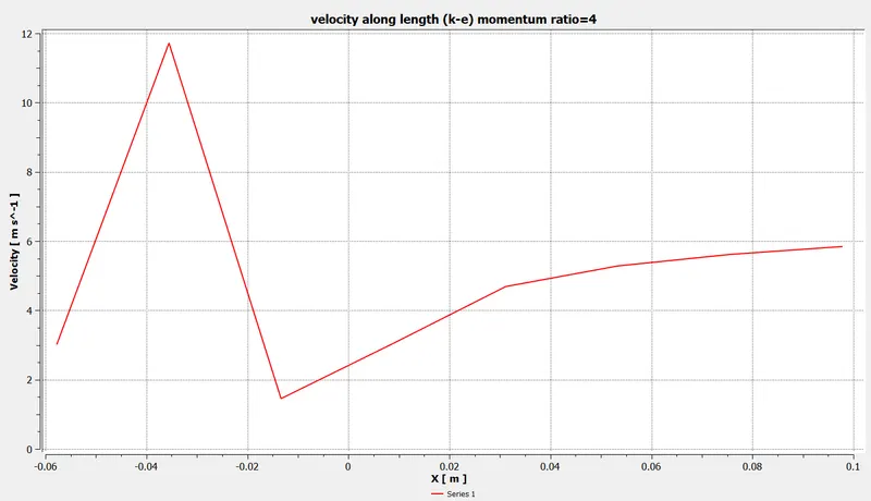
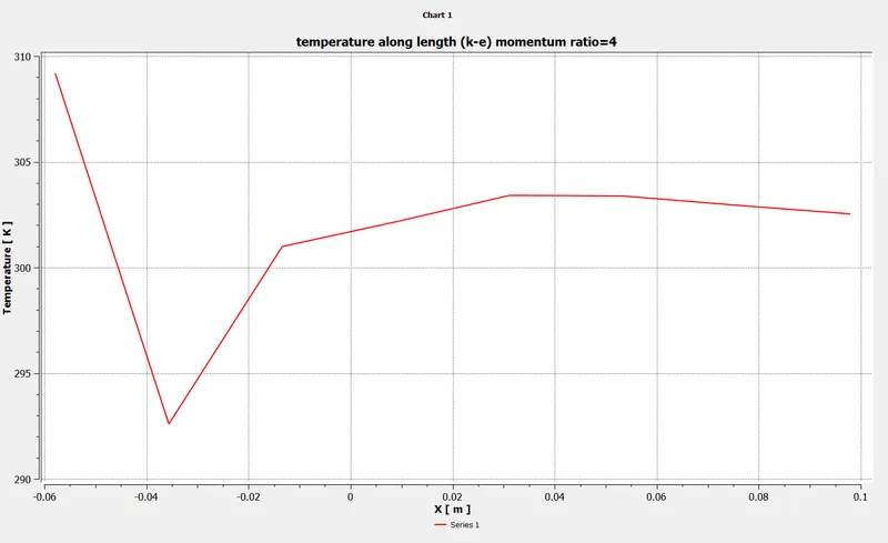
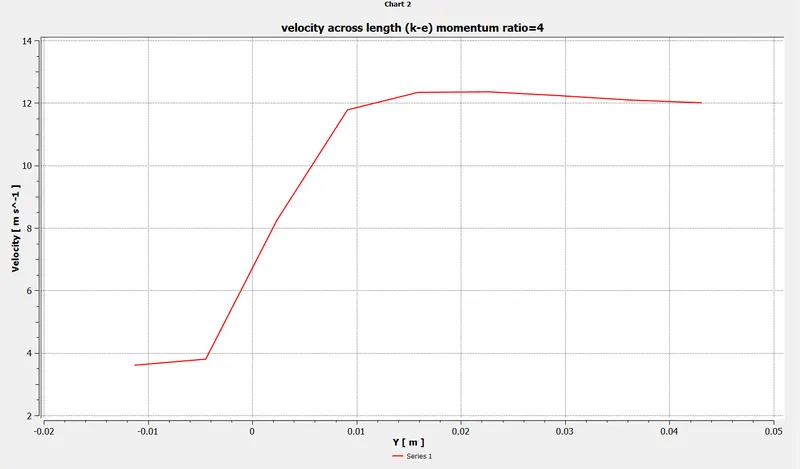
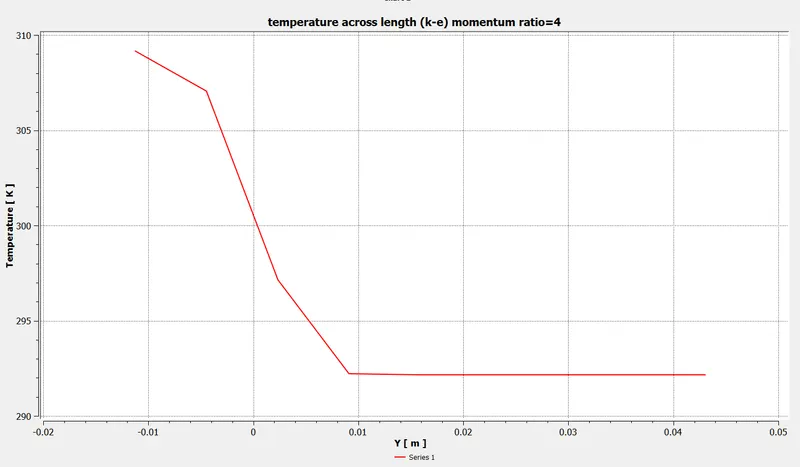
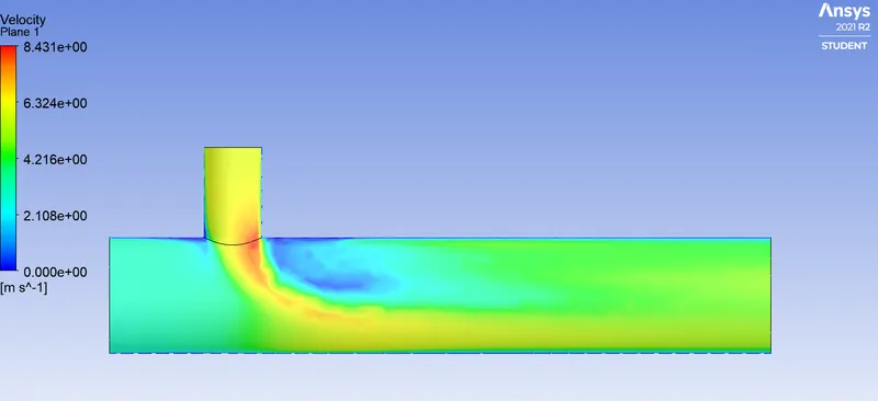
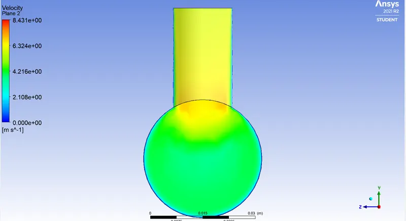
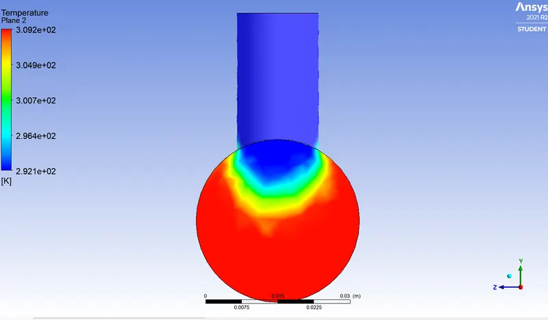
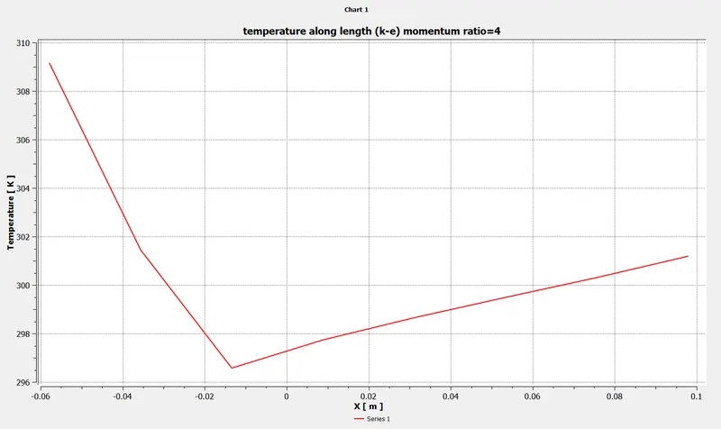
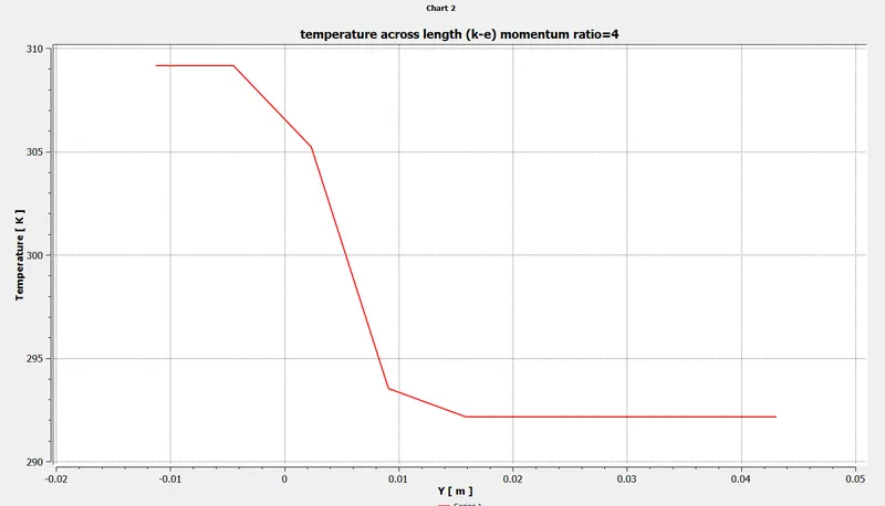
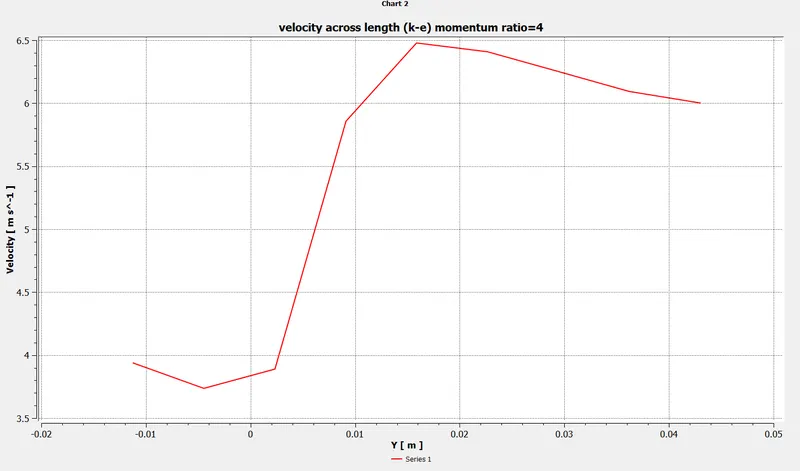
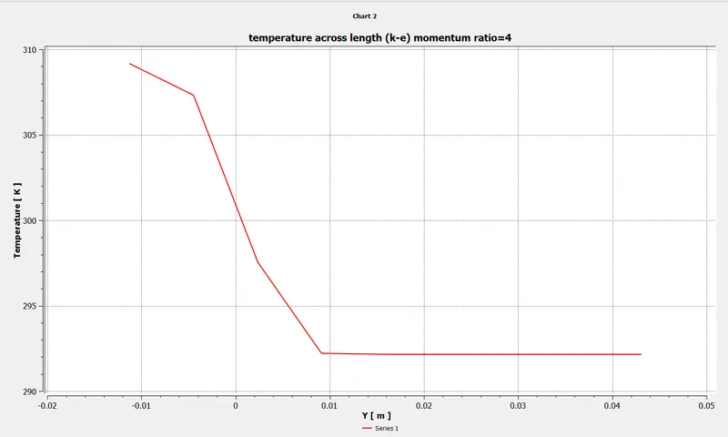
RESULTS for 3mm mesh short pipe momentum ratio=4 with k-epsilon model are shown below:

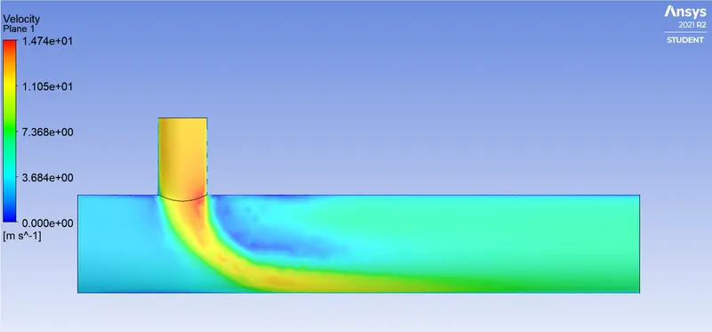
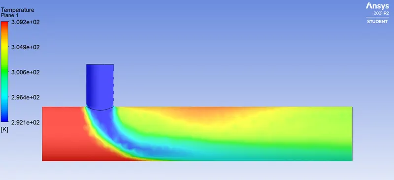
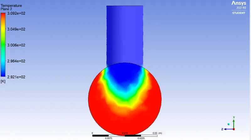
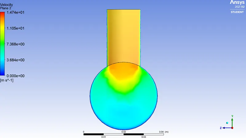
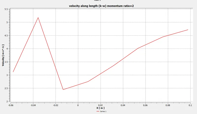
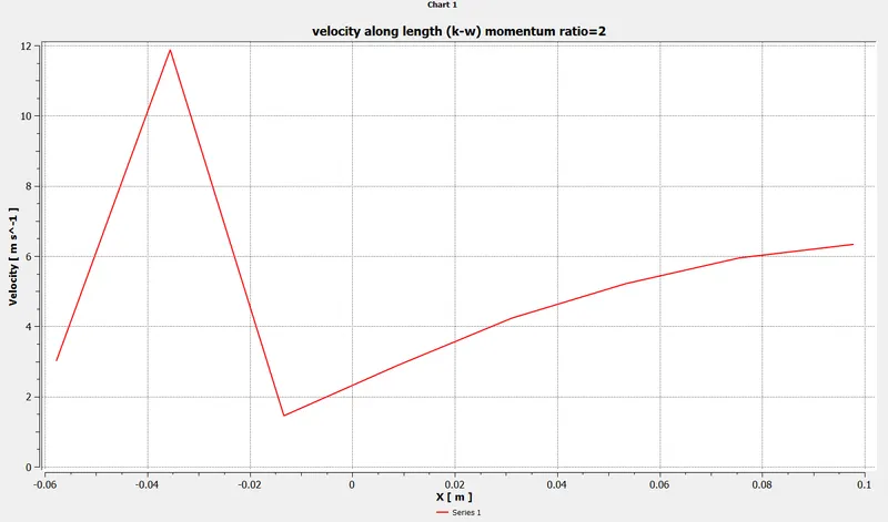
RESULTS for 3mm mesh short pipe momentum ratio=2 with the k-omega model are shown below:

Case-1 i.e short pipe was also utilized for comparing the performance of both turbulence models(k-omega and k-epsilon). K-epsilon outperformed k-omega because k-omega is used for low Reynolds number flows, k-Omega didn't converge and k-epsilon converged in fewer iterations.

K-omega is preferred in studying fluid behavior near walls, but here it is not the case. So, the k-epsilon model is recommended to study fluid far from the wall i.e. flow region, in further cases.

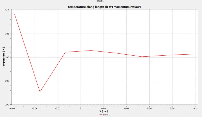
RESULTS for 3mm mesh short pipe momentum ratio=4 with the k-omega model are shown below:

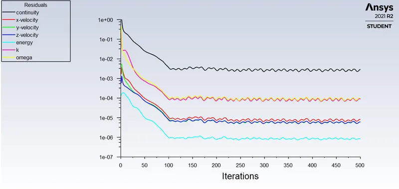
In the below analysis of short tee, the results don't converge for momentum ratio=4. But they oscillate within an upper and lower bound.

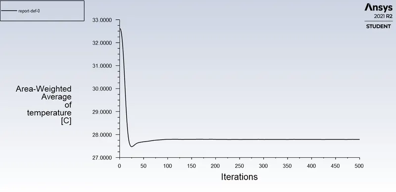
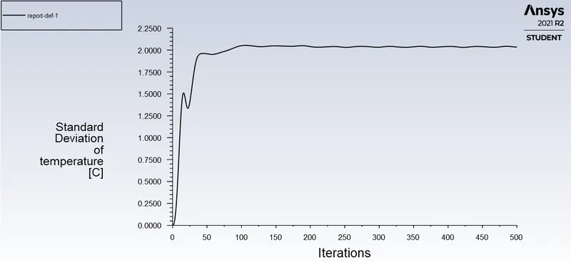
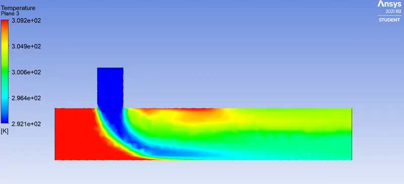
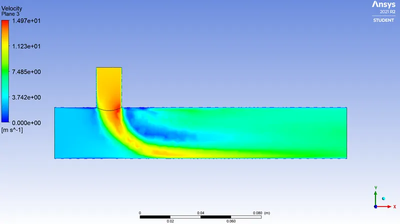
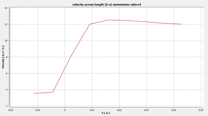
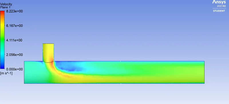
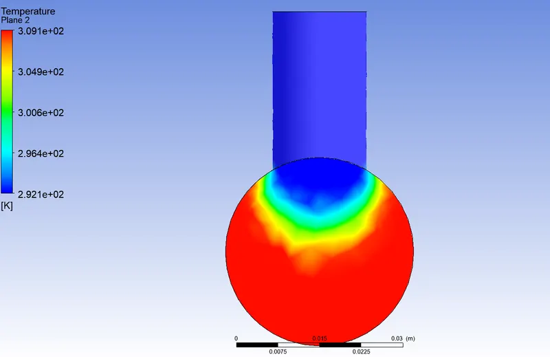
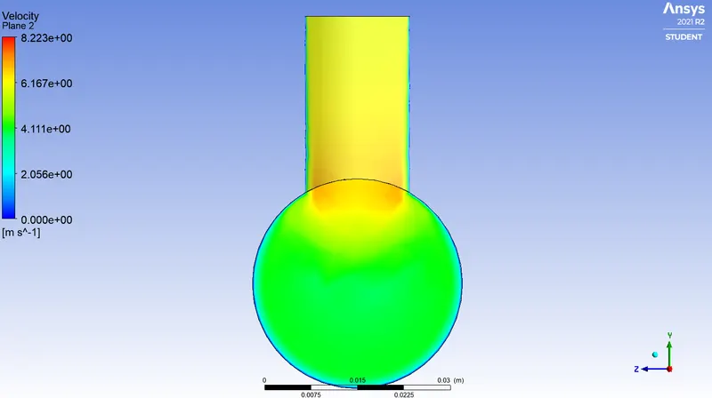
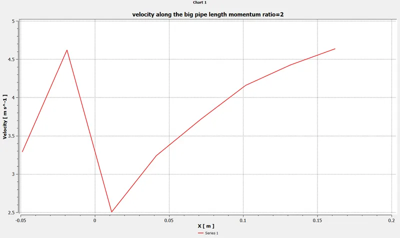
The post-processing results show the variation of temperature and velocity along and across the length of the pipe. The standard deviation reaches stability at 260iterations and also the average outlet temperature becomes 300k. The temperature and velocity show fluctuation from 309-to 302k and 3.5to 5m/s along and from 301-to 290k and 1.5to11m/s across.

FOR LONG TEE K-epsilon model along with 3mm mesh is continued.

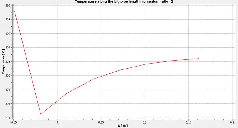
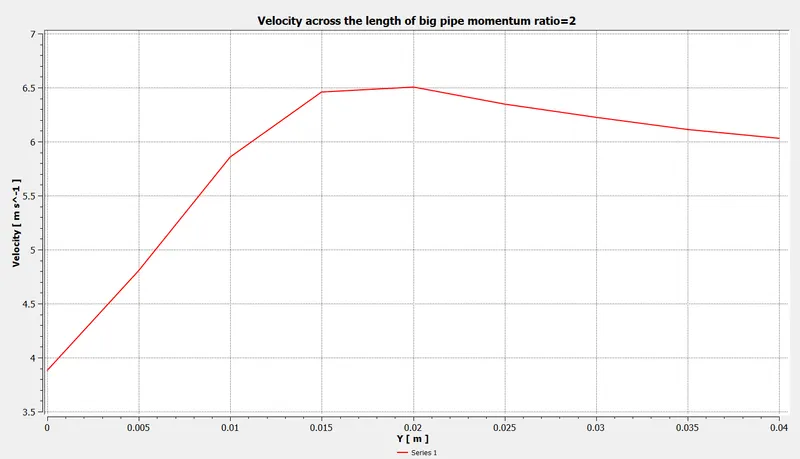
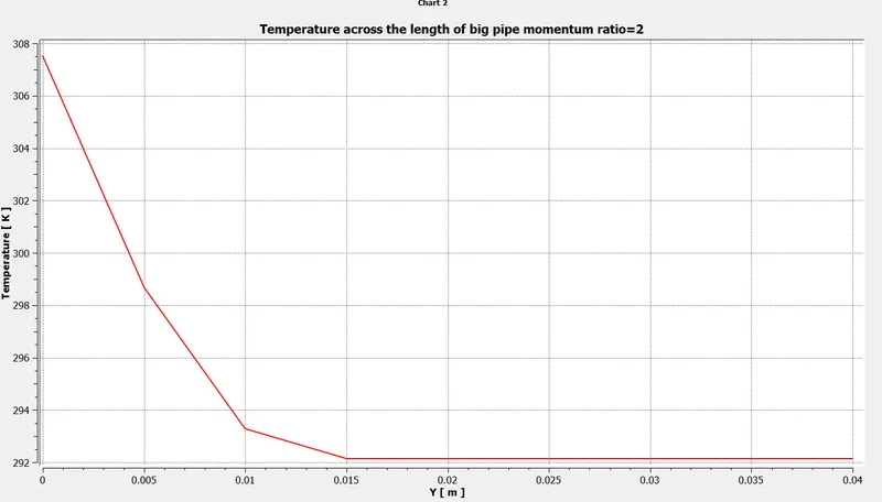
Results for momentum ratio=2.

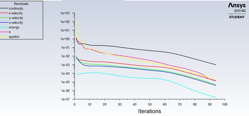
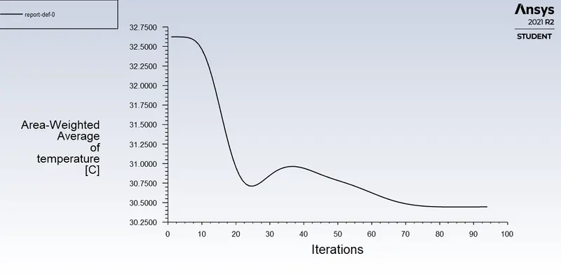
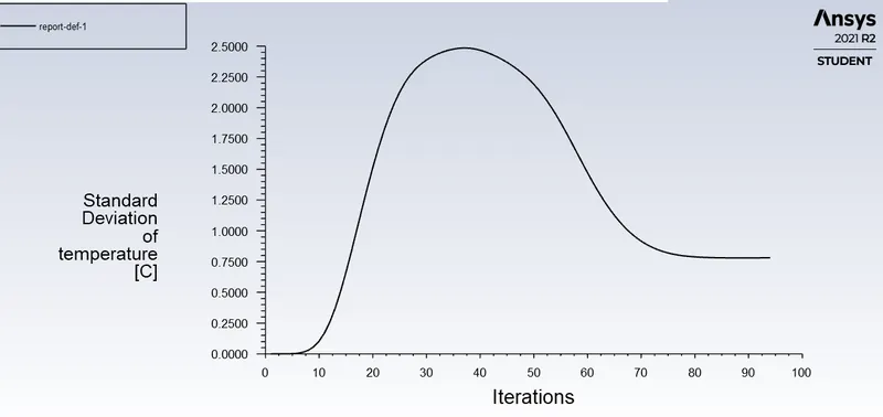
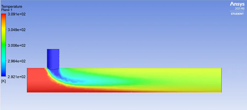
Below are the Results for the momentum ratio=4.

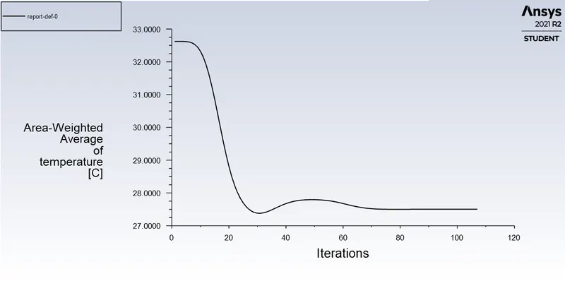
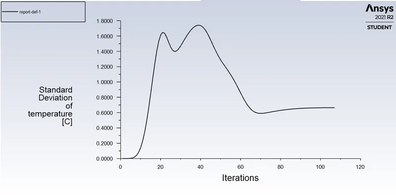
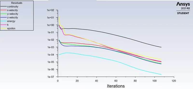
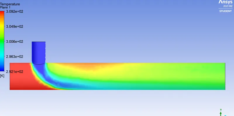
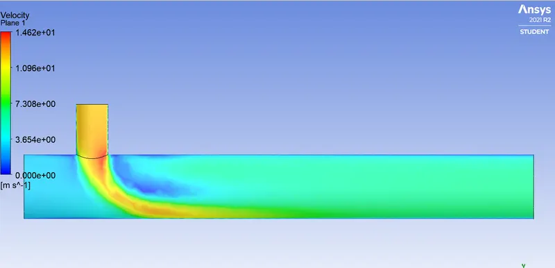
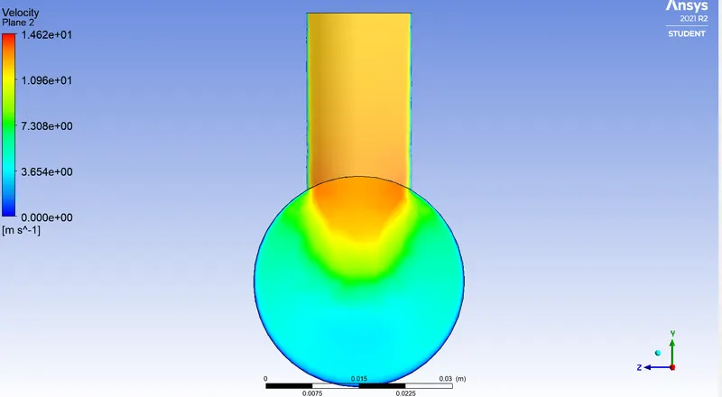
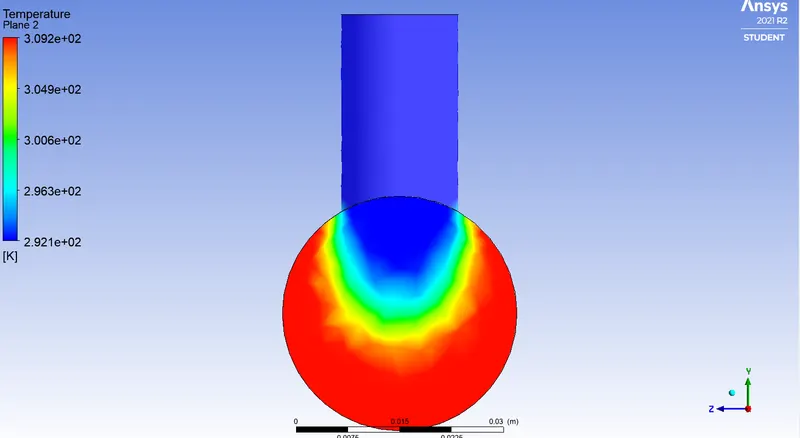
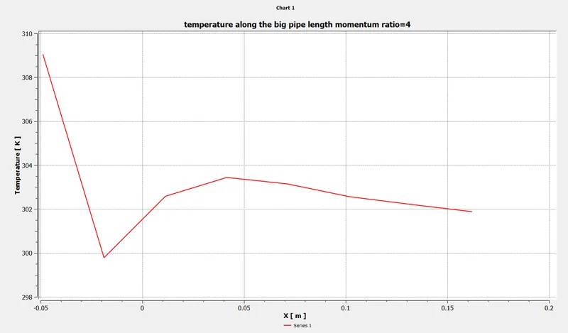
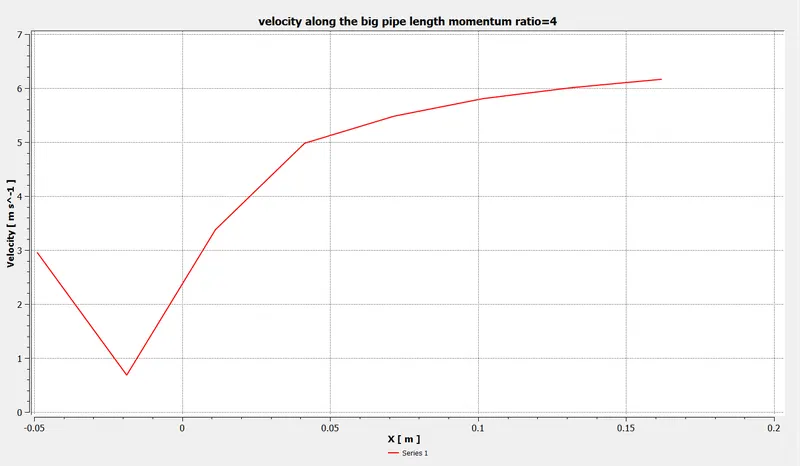
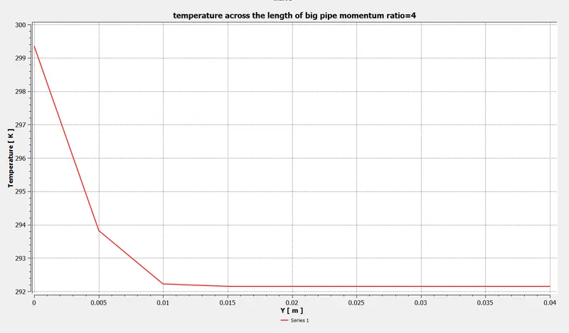
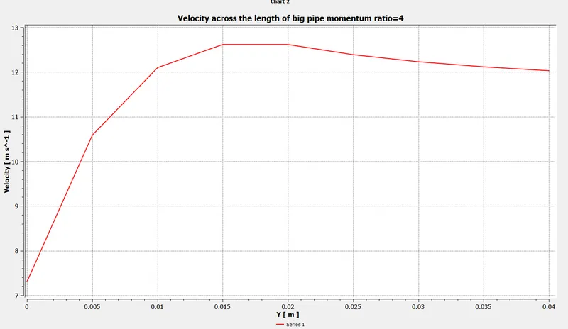
The post-processing results show the variation of temperature and velocity along and across the length of the pipe. The standard deviation reaches stability at 107 iterations and also the average outlet temperature becomes 300.5k The temperature and velocity show fluctuation from 309to 302k and 3to 6.1m/s along and from 309to 291k and 0to 12m/s across.

ANALYTICAL SOLUTION

MOMENTUM RATIO 2

Mass of hot fluid mh=`ρ.A.vh`=997⋅0.0009⋅3=`2.69kgs` mh=`ρ.A.vh`=997⋅0.0009⋅3=2.69kg/s

Mass of cold fluidmc=`ρ.A.vc`=997⋅0.0002⋅6=`1.35kgs` `mc=ρ.A.vc`=997⋅0.0002⋅6=1.35kg/s

Temperature of mixture

`Tmixture=((mh⋅Th)+(mc⋅Tc))/(mc+mh)=30.315c`

MOMENTUM RATIO 4

Mass of hot fluid

`mh=ρ.A.vh`=`997⋅0.0009⋅3`=`2.69kgsmh`=`ρ.A.vh=997⋅0.0009⋅3`=`2.69kgs`

Mass of cold fluid

`mc=ρ.A.vc`=`997⋅0.0002⋅6`=`2.3928kgsmc`=`ρ.A.vc`=`997⋅0.0002⋅6`=`2.3928kgs`

Temperature of mixture

`Tmixture=((mh⋅Th)+(mc⋅Tc))/(mc+mh)=27.46c`

On comparing the two viscous models from the analytical solution, it is seen that the k-epsilon model gives the best-predicted results. For momentum ratio 2, the numerical outlet temperature of the long tee matches with the analytical solution. Even for momentum ratio 4 it gives the same result. Considering these factors long tee is preferred due to its effectiveness in producing an accurate mixing outlet temperature. Also at a high momentum ratio, the effect of temperature and velocity distribution gets uniform.

As we can see from results also, 3mm mesh is best suited and gives more accurate and matching results from analytical solutions.

Conclusion:

• As seen in Case-1-a and Case-1-b, the temperature at the outlet drops down significantly due to the high velocity of cold air from the inlet. This is possible due to the turbulent mixing at the tee joint between hot air and cold air because of the high velocity of cold air., which is not possible in the case of low-velocity cold air.
• The temperature contour at the outlet for short tee cases shows that some of the high temperatures flow sips through without properly mixing with the flow. Whereas, in the temperature contour of long tee cases, the high temperatures flow thoroughly mixes with the rest of the flow.
• Therefore, we can recommend using the long tee and high-velocity inlet for application. This is because we have a low standard deviation in the case of long tee compared to the short tee for both momentum ratios.
• k- epsilon model predicts away from boundaries (wall) and k- omega model predicts near the wall. Even though it depends on Y+. Therefore, the K-epsilon model is majorly used for free flow away from the wall and as in this project, there is no dealing with the wall of the mixing tee for change in temperature along the length of it, so the K-epsilon model was chosen for further simulations