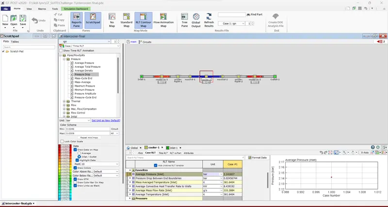
Week 1 : Exploring the GUI of GT-POWER

Aim: To explore the GUI of GT-Power, locate the listed settings, explore the intercooler tutorial, and solve a problem.

Problem Statement :

1. Explore the GUI of GT SUITE and list down modules available with a brief description. (15 marks)

2. Locate the following settings:

• Time control flag (5 Marks)
• Time step and solution control (5 Marks)
• Integrator/Solver type (5 Marks)

3. Explore the intercooler tutorial and note down all settings of:

• Run setup (5 Marks)
• Advanced setup (5 Marks)
• Plot setup (5 Marks)
• Output setup (5 Marks)

4. Problem: (50 Marks)

Given

• Diameter of cooler inlet and outlet pipe= 50 mm
• Length of the CAC= 1000 mm
• Inlet mass flow rate = 1200 kg/ h at 100 degC
• Outlet pressure 2 bar at 30 deg C

• Calculate the Average heat transfer at the Charge air cooler (CAC)
• Calculate pressure drop across CAC

Answer:

1. GT-SUITE

GT-SUITE is a single software package for system modelling and simulation in automotive, transportation, and other engineering fields. While it is built on a multi-physics platform, it provides higher level, additional value toolboxes that are especially suited to an ever-expanding collection of applications:

• Simulation of engine performance (including combustion and turbocharging)
• Examination of the engine's cylinder pressure measurements (combustion profiles)

• Vehicle dynamics (drive cycles, drivelines), the acoustics of intakes and exhausts, exhaust aftertreatment, SiL, HiL, and real-time modelling of engine, vehicle, and cooling, hybrid and electric cars, and fuel cells
• Analysis of the underhood cooling module; Cooling systems and vehicle thermal management (3-D solution with COOL3D)
• Fuel injection systems; • Hydraulic and pneumatic systems; Lubrication circuits and bearings (valve actuators, brakes, steering, power hydraulics)
• Dynamics and kinematics of the crankshaft and the valvetrain (balancing, engine bearings and mounts)
Chain, gear, and belt system dynamics; crankshaft durability and fatigue (timing drives)

Engineering apps may be found in one place with GT-Suite. Consider, for instance, the cooling circuit that includes an EGR cooler and a charge-air cooler and how it relates to engine performance. This cooling circuit may be easily studied in a single model for analysis and for the design of a combined cooling circuit and engine.

Graphical Applications within GT-Suite :

1. GT-ISE(Integrated Simulation Environment) :

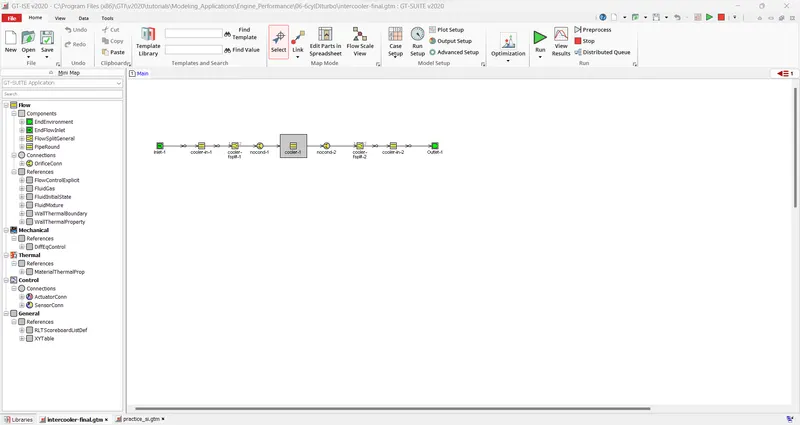
GT-ISE is the interface used to create models, define simulation parameters, and run simulations (both batch and single simulations). It is a 2-D environment in which different items are added to a project map and linked to one another, connecting the overall model.

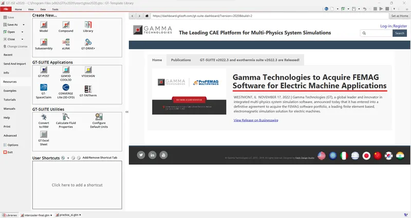
There are several examples of conducting simulations in GT-Suite that may be used as a starting point. For instance, it may be launched from the tutorials area of the file menu to mimic an intercooler. But, you may drag several template-based components into the workspace to design (or alter) your model. For instance, the current intercooler lesson now includes components for pumps and turbines.

2. GT-SpaceClaim :

The GT-SpaceClaim tool can input CAD geometry in various formats, extract volumes, and export those volumes for discretization in GEM3D. It is also possible to create and export 3D models of flow systems.

3. Gem 3D:

GEM3D is a programme that creates discretized model files for use with GT-SUITE that may be used to create 3D models of flow, thermal, and mechanical systems. In order to incorporate all of the model's intricacies, it offers the option of building the model in a 3D environment. Moreover, it has powerful discretization logic that can convert the 3D model into a model file that the GT-SUITE programme can use. Every system with parts such as pipes, mufflers, manifolds, air boxes, heat exchangers, under the hood, inside the cabin, batteries, crankshafts, etc. may be constructed using GEM3D.

4. GT-Post :

It is possible to plot, examine, and alter data produced by a GT-SUITE simulation or by an external source using the robust data analysis tool GT-POST. It provides a data analysis solution that is more effective than spreadsheet software in general. The results shown in GT-POST are updated automatically and instantly when a model is altered and a simulation is performed by using data pointers.

2. Locating the settings :

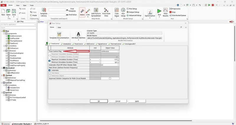
1. Time control flag

The simulation runtime and time-controlling variables are configured using time-control settings. For every simulation, the properties in this folder must be specified.

The global simulation type—whether it is periodic or continuous—is defined by the time control flag.

For models that include a periodic occurrence, the term "periodic" is used (ex: engine cylinder). A periodic simulation's simulation time may be given either in cycles or in time, depending on which is most practical.
Continuous means that there are no periodic events in the simulation, hence there is no need to keep track of the findings in relation to a cyclic angle.

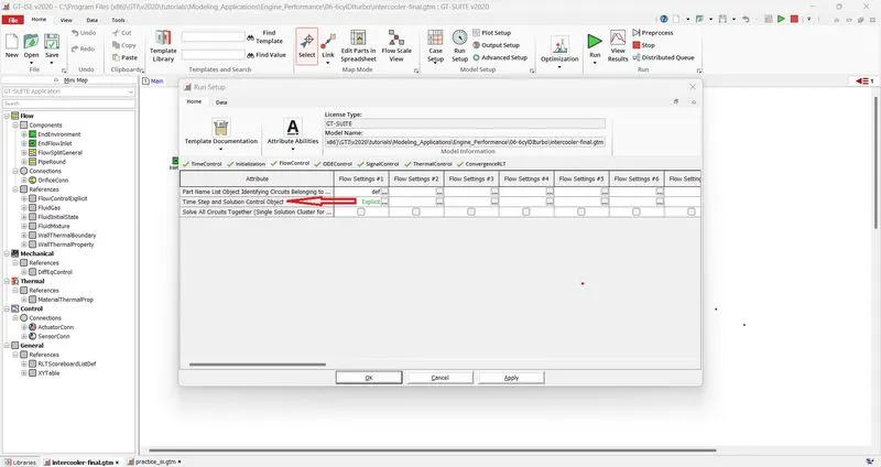
2. Time step and solution control

The numerical parameters for the explicit, implicit, or quasi-steady flow solver are defined using them.

3. Integrator/ Solver type

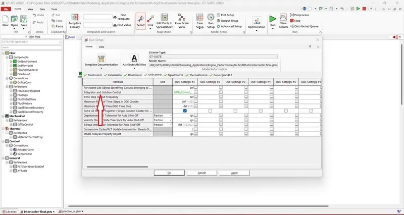
Time-marching of all ODEs, including those in mechanical, electrical, and magnetic libraries, uses the integrator/solver type. Depending on the application, many schemes are accessible and chosen.

For variable order accuracy, the explicit Adams-Bashforth-Moulton predictor-corrector integration technique.
5th order accurate explicit Runge-Kutta integration technique.
A 2nd order accurate implicit trapezoidal integration technique.
Second order accurate implicit Hilber-Hughes-Taylor integration scheme.
Implicit 3-order accurate 2-stage Radau integration technique.
Implicit 5-order accurate 3-stage Radau integration technique.
Implicit 5-order accurate 3-stage Spectral Deferred Correction (S.D.C.) integration technique.

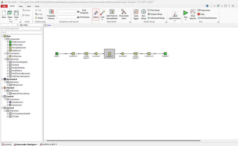
3. Intercooler simulation tutorial :

1. RUN SETUP

In this settings, the simulation parameters like simulation run time, etc are specified.

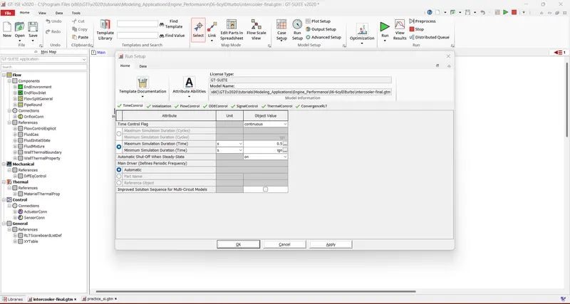
a) Time Control:

The simulation runtime and time-controlling variables are configured using time-control settings. For all simulations, the properties in this folder must be specified.

As there are no periodic events in this model, the time control flag is set to continuous.

The simulation will end automatically if all steady-state convergence requirements have been satisfied, according to the setting Automatic Shut-Off When Steady-State - ON.

- OFF signifies that there will be no automated shut-off and that the simulation will run for its full length.

For continuous models, the maximum simulation duration property is used to regulate the length of the simulation, and it may also be used for periodic models that need to run for a certain amount of time (i.e. a transient event).

If the simulation has achieved steady-state and the Automatic Shut-off When Steady State flag is set to on, the simulation may end before the maximum simulation period.

When the Automatic Shut-off When Steady State flag is set to on, the Minimum Simulation Duration (Time) property may be used to make the simulation continue for a certain amount of time.

When the Automatic Shut-off While Steady State flag is set to off, this property will be ignored.

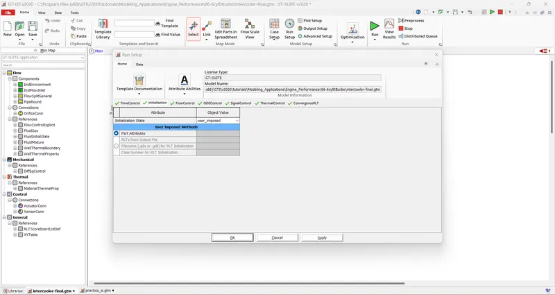
b) Initialization :

The beginning circumstances for the simulation will be enforced according to the specifications specified in this folder. During time=0.0 of the simulation, each state variable has to be initialised. For instance, initialization requirements include initialising flow components with pressure, temperature, and composition; flow connections with velocity or mass flow rate; shafts with rotational speed; other mechanical parts position; and certain control components with a "State" value.

The state variables for each new case of the simulation will be initialised with values imposed by the user, as indicated by the initialization state: user imposed. The values for the user-imposed circumstances may either originate from the characteristics for the starting pressure, temperature, velocity, and speed, which are given in each component of the model, or from the outcomes of a prior simulation.

Feature Qualities With this selection, the properties listed in the model map portions for each example will be used to initiate the simulation. User imposed initialization is the sole condition in which this option is accessible.

c) Flow control:

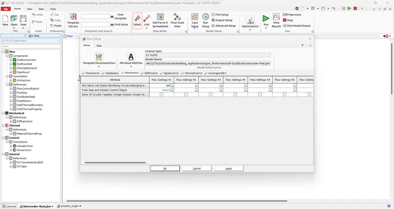
This folder is used to provide solver parameters relevant to simulating the flow for separate flow "circuits" inside the model. A set of linked flow components that normally share the same fluid constitutes a circuit.

One flow circuit will be present in several simulations. The Part Name List Object Identifying Circuits Belonging to Column in this instance simply has to be set to "def," since it is only essential to utilise the first column.

d) ODE Control:

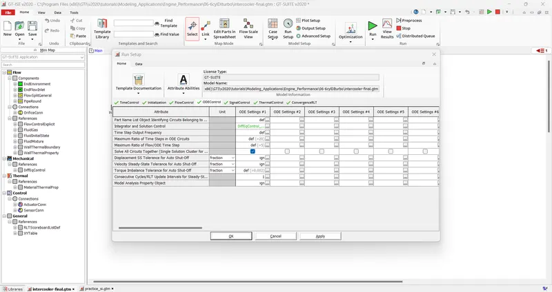
Throughout the model, separate "ODE circuits" are defined in this folder together with the solver parameters for each of these circuits. A set of linked mechanical, electrical, magnetic, or control components may make up an ODE circuit. Even if the model has several mechanical or control circuits, for many simulations, the prefilled values in this folder won't need to be changed. Nonetheless, the folder offers the option to create distinct circuits if necessary, as well as to modify the solver ODE parameters for any ODE circuits.

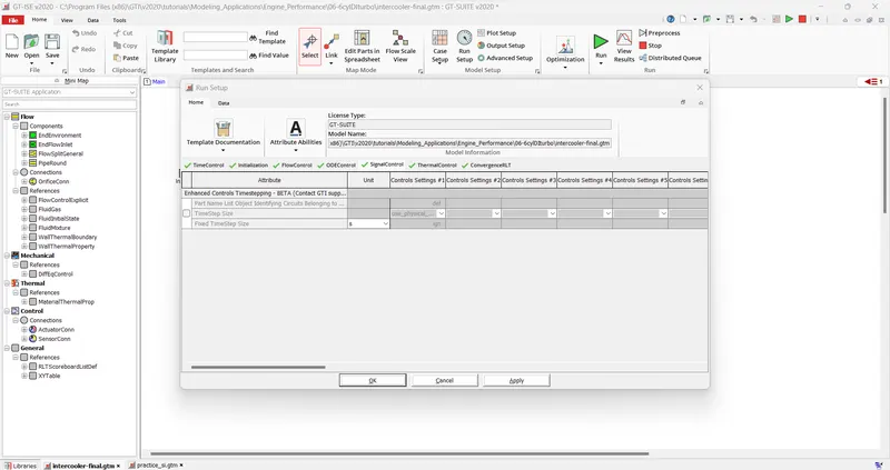
e)Signal Control:

f)Thermal Control:

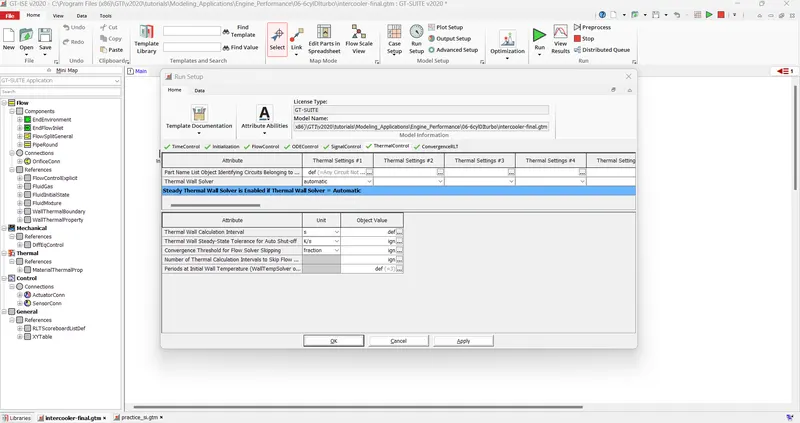
Just the thermal wall (structural) solver, which includes the aftertreatment, finite element objects, thermal mass/block/node, and the wall material of pipes and flowsplits, is controlled by this folder. The fluid's thermal calculation, which cannot be turned off, is not within the control of this folder.

The Thermal Wall Solution for pipe/flowsplit walls and other thermal masses will be automatically chosen when Thermal Wall Solver - automated is selected. Based on the option for Automatic Shut-Off During Steady-State from Run Setup -> Time Control, the automated solver will decide between steady and transient. The stable Thermal Wall Solver will be utilised if auto shut-off is set to "on". The transitory Thermal Wall Solver is utilised if auto shut-off is "off".

g)ConvergenceRLT:

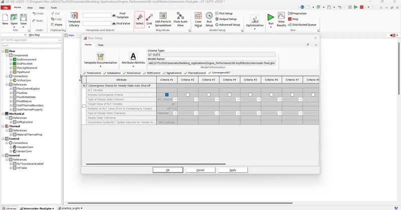
This folder can optionally be used to impose one or more steady state criteria (up to a maximum of 10) that depend on RLT variables in a simulation.

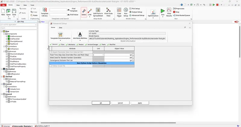
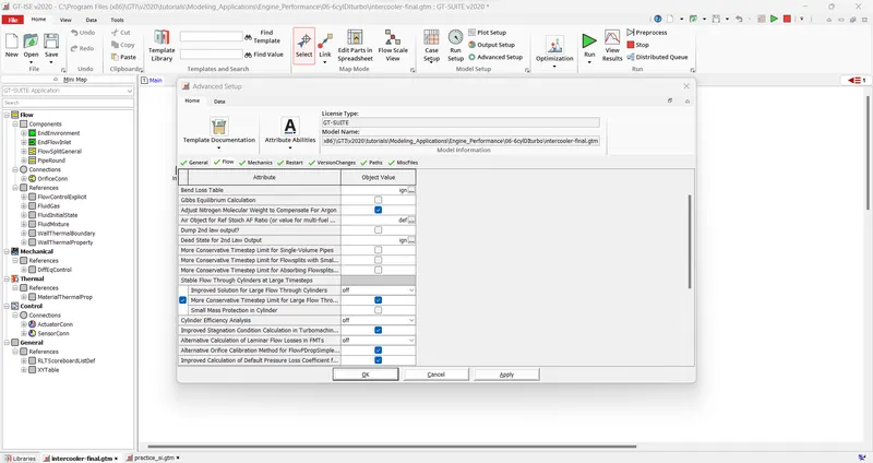
2. Advanced Setup :

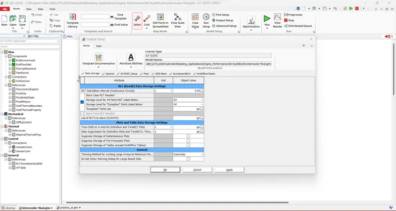
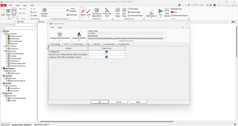
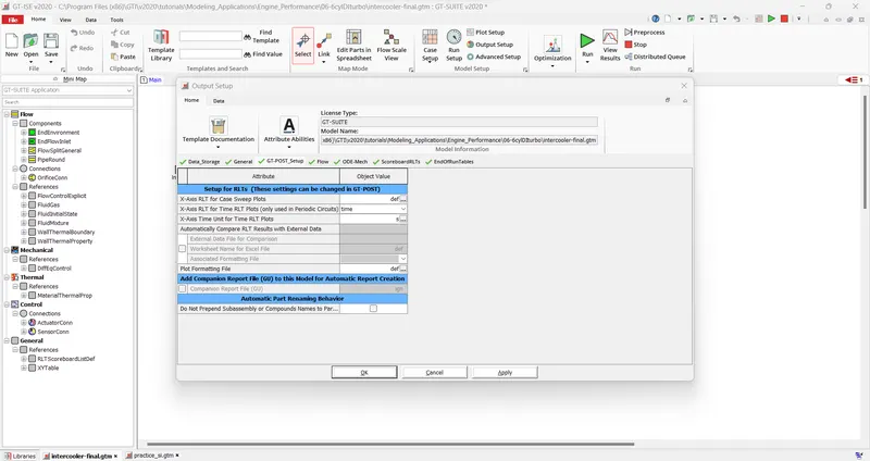
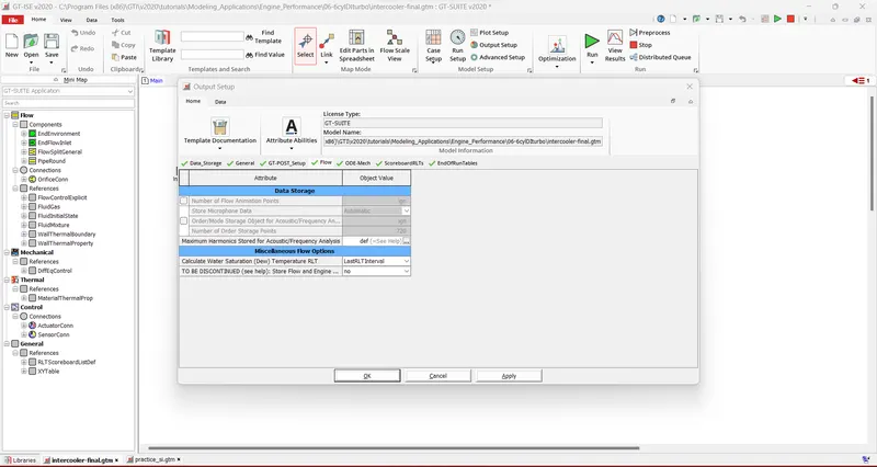
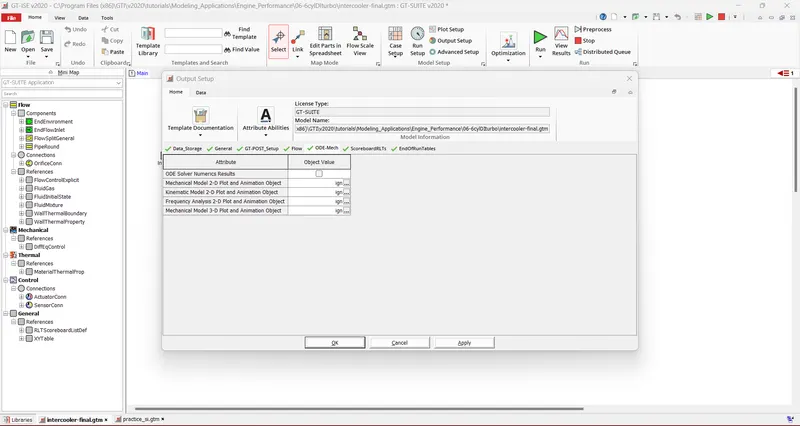
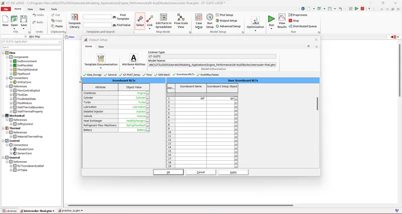
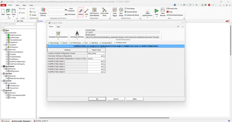
3. Output setup :

In this setting, the parameters regarding the outputs are specified.

a) Data storage:

In scenarios when not all of the information from GT-SUITE is useful, this folder may be used to opportunistically conceal some of the content. These choices may be particularly helpful for models that have a lot of components, spanning a lot of cycles, or have a lot of instances.

4. Plot Setup:

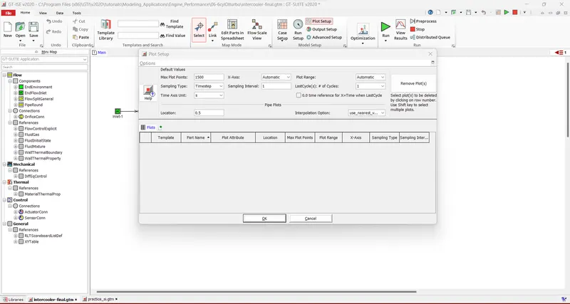
The parameters pertaining to the plots are described in this context.
The "Run" pull-down menu's Plot Setting option offers the user a number of choices to modify how the plots are requested.

4. Problem:

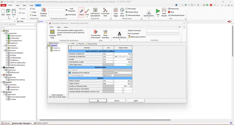
Given

• Diameter of cooler inlet and outlet pipe= 50 mm
• Length of the CAC= 1000 mm

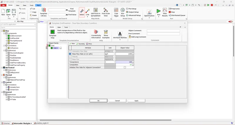
• Inlet mass flow rate = 1200 kg/ h at 100 degC

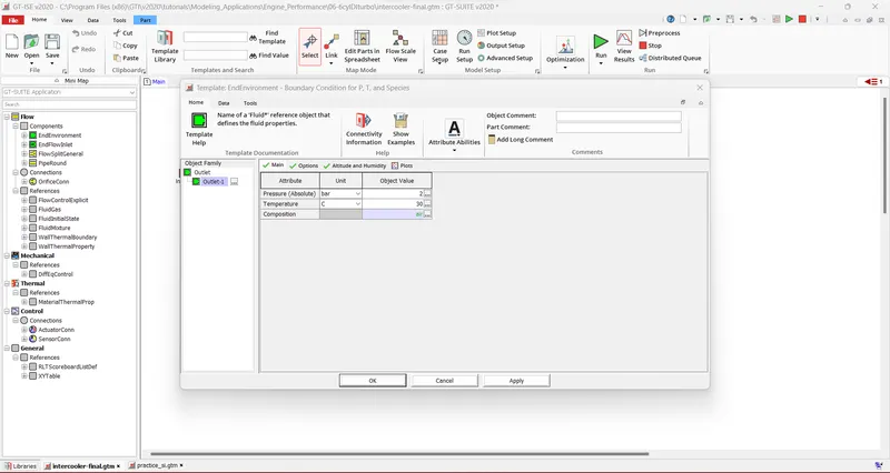
• Outlet pressure 2 bar at 30 deg C

Results:

• Calculate the Average heat transfer at the Charge air cooler (CAC) - 8.44KW

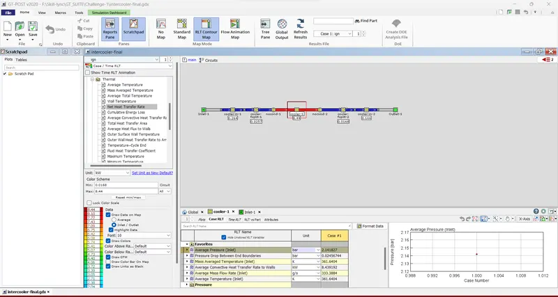
• Calculate pressure drop across CAC - 0.0309 bar