Week 1: Channel flow simulation using CONVERGE CFD
Week 1: Channel Flow Simulation using CONVERGE CFD
Aim:
The main aim of the project is to set up a 2D Channel Flow simulation in CONVERGE CFD software in which the simulation is set up with three different meshing parameters assigned with certain inlet and outlet boundary conditions.
Channel Flow:
The flow that are surrounded by boundaries are mostly internal flows where the flow occurs because of the pressure gradient. The internal flow applications mostly arise with the rectangular or circular cross section in which they are in contact with the rigid boundaries. The fluid flow in the closed channel is covered and has no free surface. Velocity is maximum at the centre of the flow and reduces to zero at the pipe wall. Velocity distribution is symmetrical about the closed channel axis in channel flow.
Flow assumptions:
- Incompressible flow (Pressure is Constant).
- Viscosity is assumed to be constant.
- Fully developed flow
- Steady flow
- Two dimensional flow
- Body force is not considered
- No heat transfer occurs
Mathematical Modelling:
Any physical phenomenon can be represented as a mathematical model that gives us the information about the process that is going on the domain. These mathematical modelling basically represents the information about the behaviour of the process through governing equations.
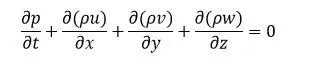
Governing equation consists of partial differential equations:
- Continuity equation:
- Momentum equation:



For this channel flow case we are assuming that there is no heat transfer and that the temperature remains constant which leads us to ignore energy equation and consider only the continuity and the momentum equations for each axis direction. By considering certain conditions we are left with the 4 unknowns. These equations can be solved as a system of linear equations using an iterative solver.
Geometry:
- The CONVERGE CFD software is installed by following the steps.
- The geometry is created by using the following steps.
- First of all open the CONVERGE CFD software and open a new project.
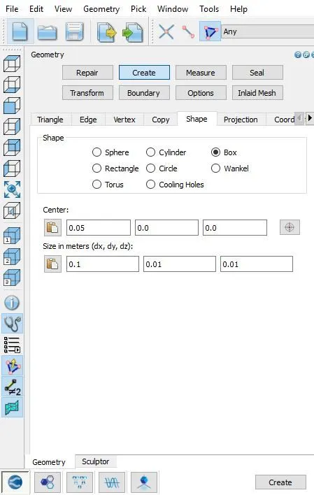
- Geometry-->Create-->Shape-->Box-->Enter the dimensions of the box to be created and then click on create.
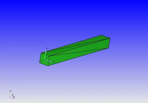
3D Model:
- Forming Boundaries: To create the boundary regions click on Boundary-->Flag-->Click on the "+" symbol to create boundaries.
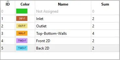
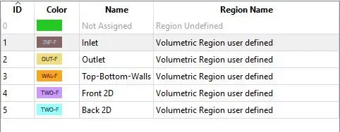
- The boundaries can be created in two ways. The first way is by entering the unique boundary id and boundary name manually. The second way is by using the "Create multiple boundaries" option which enables us to create multiple boundaries at once. A total of 5 boundaries are created for our case. After the boundaries are formed, it is named as inlet, outlet, Top-Bottom-walls, Front 2D, Back 2D respectively. While assigning the specific regions to the named boundaries we have to make sure that we have selected the desired region's triangle.
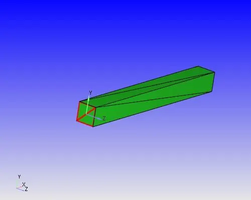
- The named boundaries are as follows,
- Then Click on the Normal Toggle option and click on any of the triangle which shows the normal opposite to the direction of the fluid flow and click apply.
- Then click on Options-->Visibility-->Geometry Bounding Box to create a boundary line across the geometry.
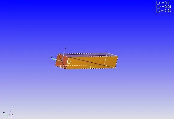
- TO ensure that the geometry is clean click on the Diagnosis tab and click Find option.
- All the parameters that got checked shows the green colour tick mark.
Case Setup:
For setting the case for our model the following steps are done.
- Click on Case Setup--> Begin Case Setup option and a pop up window appears. In that choose Time-based, since we are solving for steady state channel flow setup.
- Then click on Materials which is present in the right side of the window that is case setup tree, uncheck the Reaction mechanism since there is no chemical reaction taking place in our channel flow case and select the Predefined mixtures as Air.
- Click on the Gas simulation and Global Transport parameter and retain the same values.
- Click on Species and then add O2 and N2.
- Click on Run Parameters and under the solver tab choose the solver as Steady-State Solver. Set the simulation mode to Full Hydrodynamic and the gas flow solver as compressible
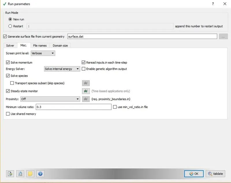
- Then under "Misc" tab check the Steady-state monitor and uncheck the use shared memory boxes.
- Then coming to Boundary Conditions click on Boundary--> Inlet -->Specify the inlet pressure value as 100001 Pa and select the predefined mixture as Air which contains N2 of 77% and O2 of 23% and then under the Temperature boundary condition choose specified value and allocate the temperature value with 300k.
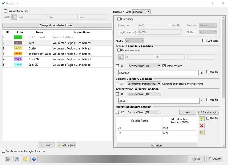
- And at the Outlet assign the pressure value with 100000 Pa and add the species.
- Assign the Top-Bottom-Walls with the Boundary type as Wall and assign with no-slip condition.
- The Front 2D and Back 2D boundary regions are assigned as TWO_D.
- Then under the Simulation Parameter --> Run Parameters select the Steady-state monitor --> add config and then click on add option to add the variables to be monitored.
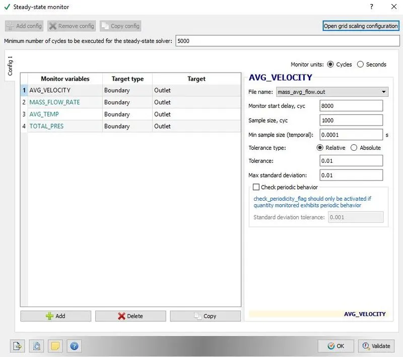
- The Monitor start display is a parameter that ensures that the simulation runs for a certain number of cycles before the variable can be monitored. This is especially useful in transient simulations when we want the solution to run for a particular amount of time before checking the convergence, if the steady state results are also required.
- Sample size denotes the number of cycles or seconds over which the variable is checked to see if the solutions have converged.
- Then under the Simulation Time Parameters assign the End time and look after the Maximum Convection CFL limit and assign with 1.
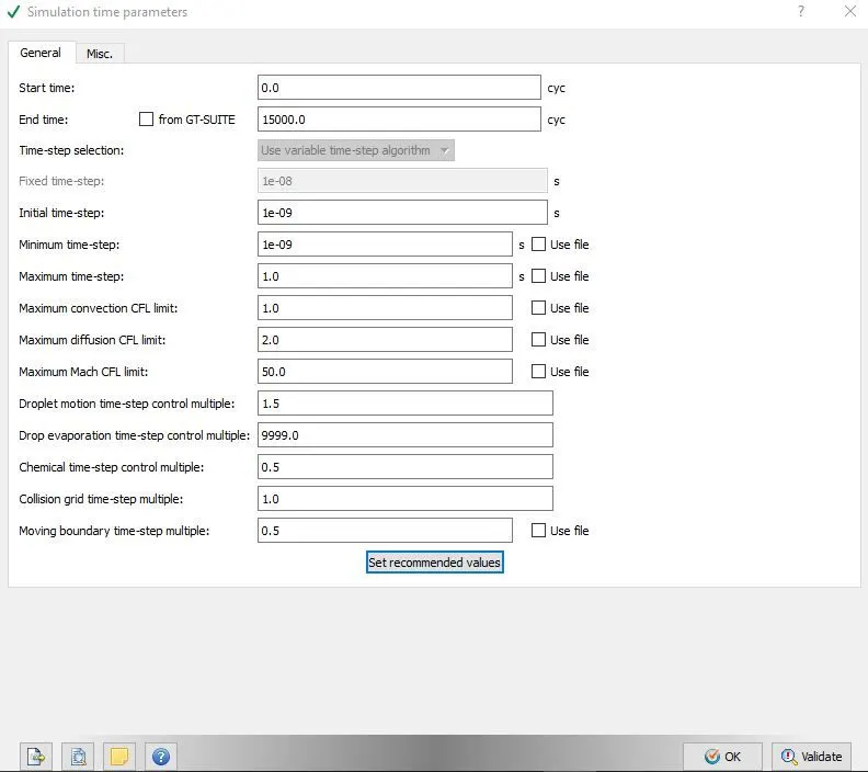
- Then click on Solver Parameters [Steady-state] --> Equations --> Pressure --> Make sure that the Preconditioner is set to None. Then under the Steady-state solver control assign the maximum convection CFL limit (final stage) to less than 1 --> Click on Validate --> Click on OK.
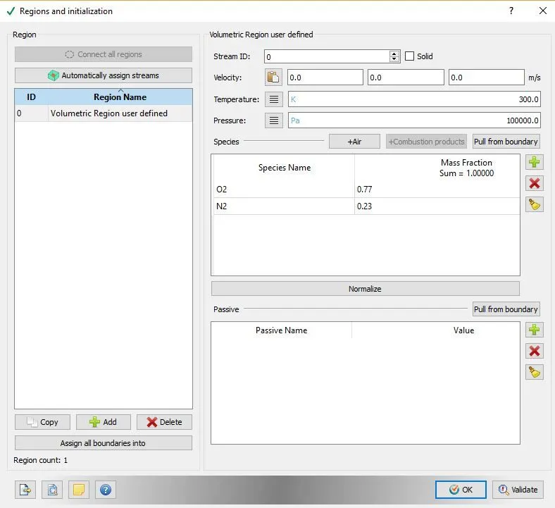
- Then under the Initial conditions and Events --> Regions and Initialization --> add a region and rename it as Volumetric Region User Defined by using the F2 option and assign the pressure value to 100000 Pa and click on Air as species. In this the O2 mixture is assigned with 77% and N2 is assigned with 23%.
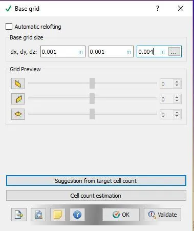
- Then in the Grid Control parameter --> Base Grid --> Enter the size of the grid.
- Then under Output/Post-Processing --> Post Variable Selection --> Add the Mass fraction with O2 and N2
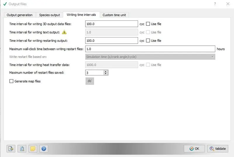
- Then under the Output files --> Writing time intervals --> set the time interval for writing 3D output data files and time interval for writing restarting output.
- Then under the Boundary assign the region name for the named boundaries.
- Click on Validate and check for errors.
- And at last export the input files to the folder that is to be solved.
Mesh Refinement:
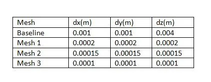
In this numerical simulation, mesh refinement was carried out by utilizing values for different mesh sizes, as described in the following table as part of each individual case setup and was entered into corresponding columns representing the 'base grid' sub option in the 'Grid Control' settings under the 'Case Setup' tree to compare the results obtained for the velocity magnitude values at the outer and pressure drop across the entire domain.
Case 1:
In the case 1 the size of the mesh is assigned with 2e-4.
Mesh:
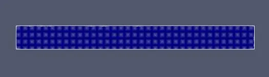
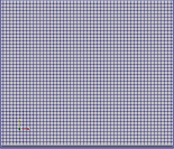
The total no of cells in the above mesh is 25000.
Velocity Contour:
Pressure Contour:
Velocity Plot:
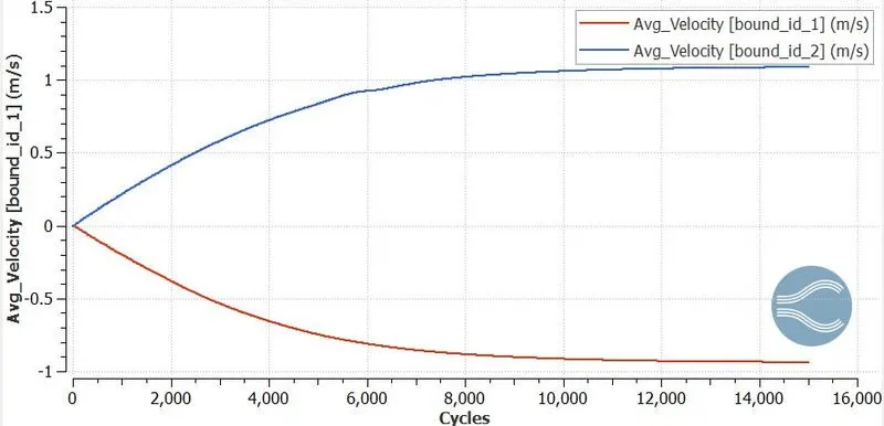
In the above Velocity plot, we easily observe that at the inlet, velocity is gradually decreasing as there is an increase in pressure at inlet.
At the outlet we observe that the velocity is gradually increasing due to decrease in pressure.
Pressure Plot:
Total and Static Pressure at inlet:
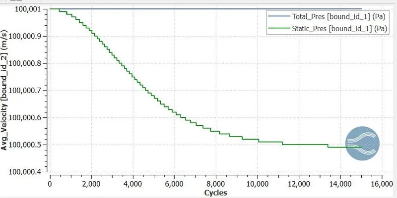
At the inlet the we observe that initially total and static pressure remains the same. As the cycles passes the static pressure is decreasing due the increase in dynamic pressure.
The total pressure is given as,
Total Pressure = Static Pressure+Dynamic Pressure.
After certain cycles we could observe that the static pressure decreases rapidly because of increase in speed of the fluid flow.
Total and Static Pressure at outlet:
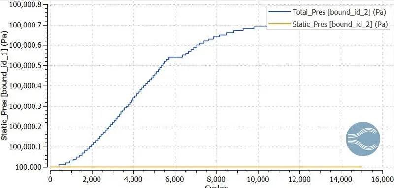
In the outlet the total pressure is increased because of the increase in dynamic pressure.
Mass Flow Rate:
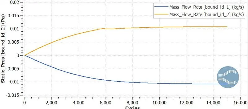
Mass flow rate is defined as the mass of the substance which passes per unit time. Here the mass flow rate at the inlet is decreased due to high pressure and low velocity.
Total Cell Count:
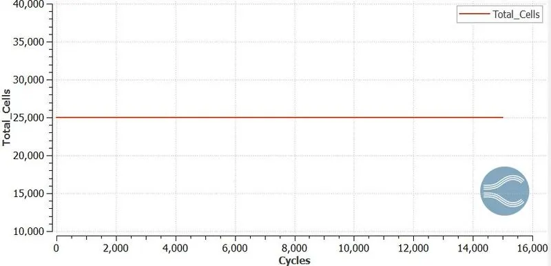
As we have fixed the mesh size to be 2e-4 there are total of 25000 cells created.
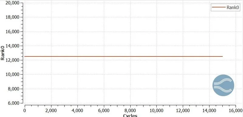
Rank0:
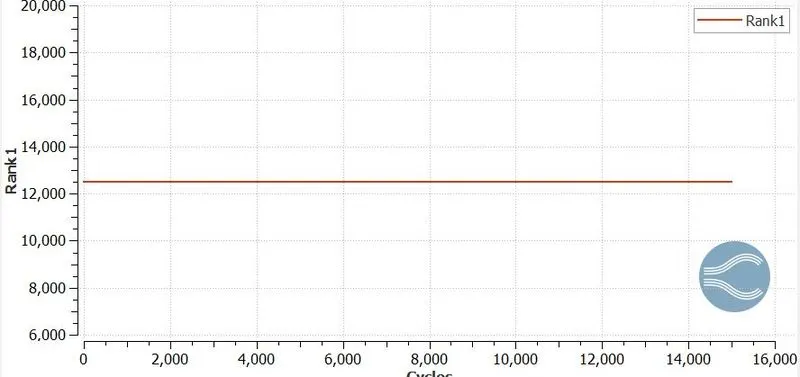
Rank1:
Animation for Case 1:
Case 2:
In the case 2 the size of the mesh is assigned with 1.5e-4.
Mesh:
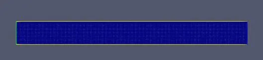
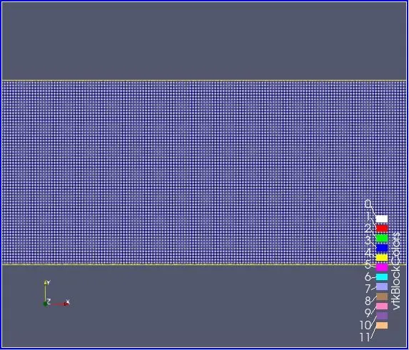
The total no of cells in the above mesh is 45420.
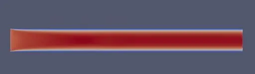
Velocity Contour:
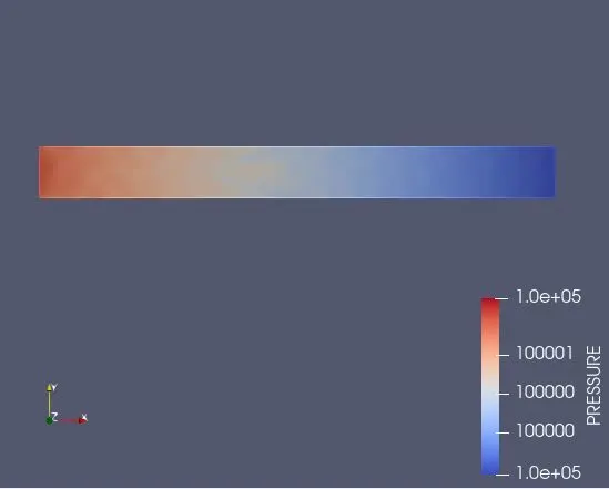
Pressure Contour:
Velocity Plot:
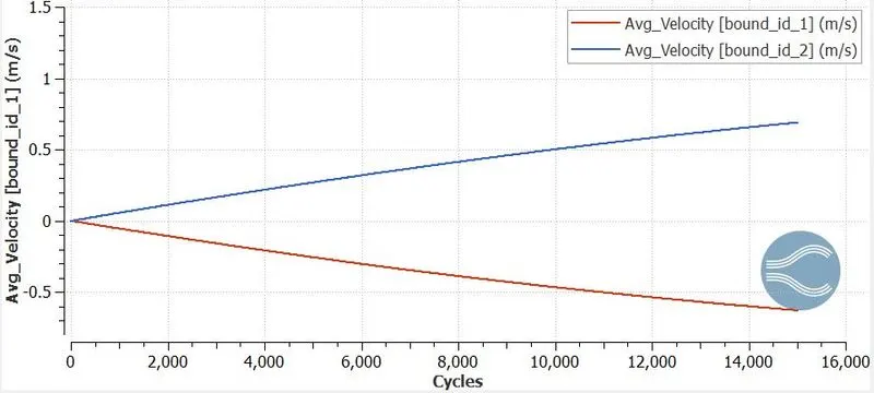
In the above Velocity plot, we easily observe that at the inlet, velocity is gradually decreasing as there is an increase in pressure at inlet.
At the outlet we observe that the velocity is gradually increasing due to decrease in pressure.
Pressure Plot:
Total and Static Pressure at inlet:
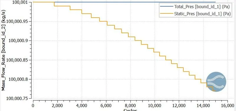
At the inlet the we observe that initially total and static pressure remains the same. As the cycles passes the static pressure is decreasing due the increase in dynamic pressure.
The total pressure is given as,
Total Pressure = Static Pressure+Dynamic Pressure.
After certain cycles we could observe that the static pressure decreases rapidly because of increase in speed of the fluid flow.
Total and Static Pressure at outlet:
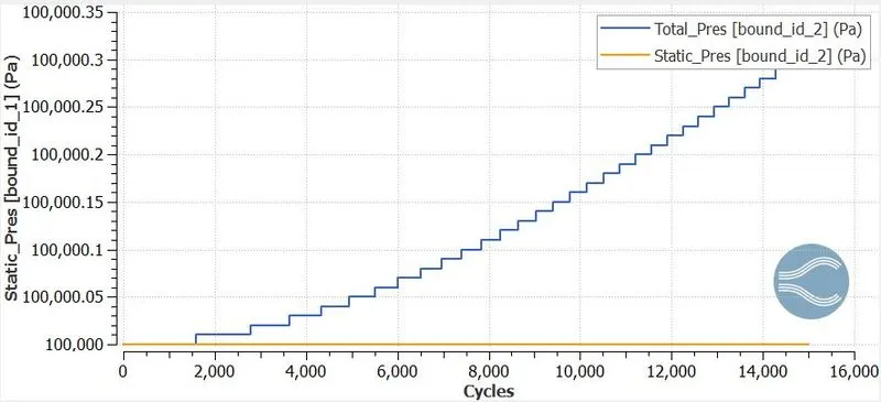
In the outlet the total pressure is increased because of the increase in dynamic pressure.
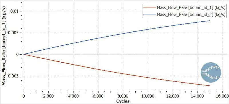
Mass Flow Rate:
Total Cell Count:
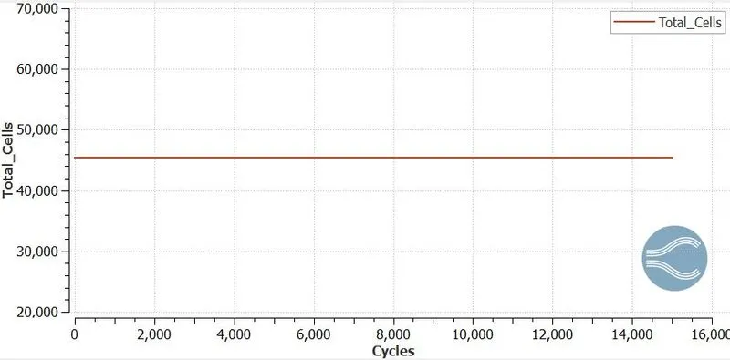
As We have fixed the mesh size to be 1.5e-4 there are total of 45420 cells created.
Rank0:
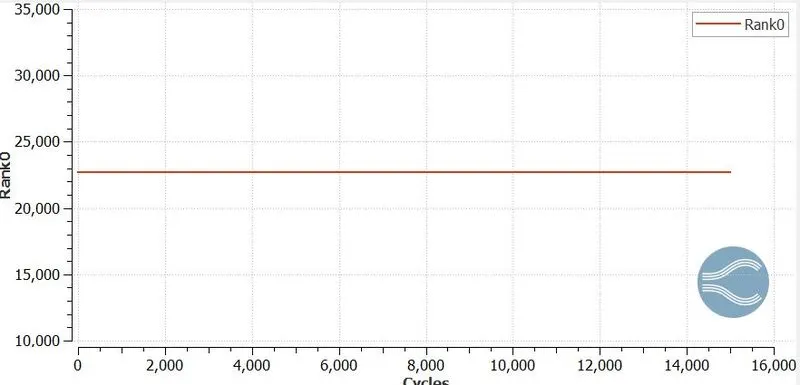
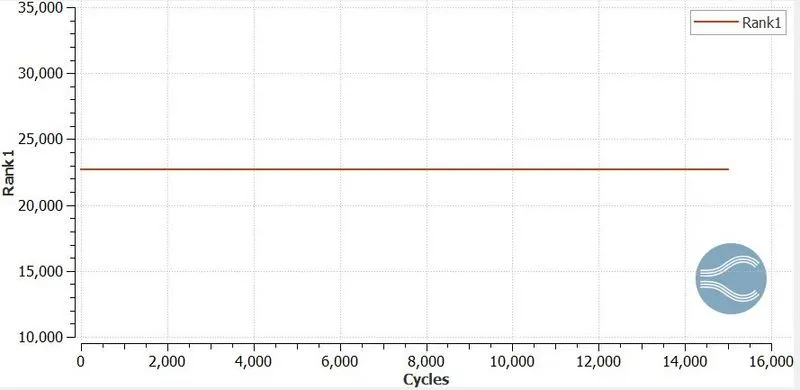
Rank1:
Animation for Case 2:
Case 3:
In the case 3 the size of the mesh is assigned with 1.0e-4.
Mesh:

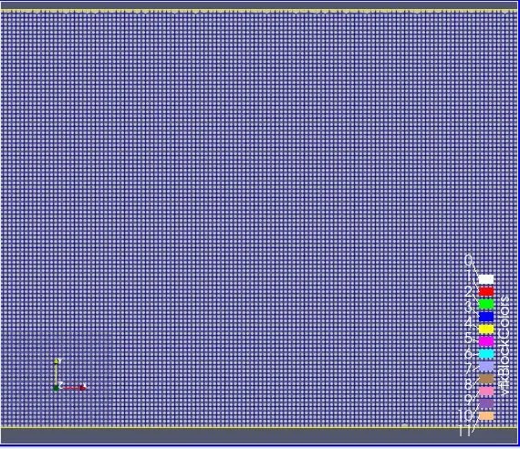
The total no of cells in the above mesh is 100000.
Velocity Contour:
Pressure Contour:
Velocity Plot:
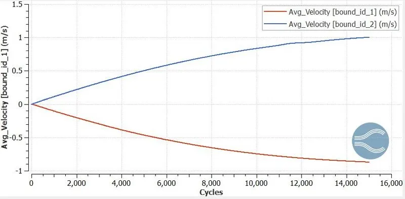
In the above Velocity plot, we easily observe that at the inlet, velocity is gradually decreasing as there is an increase in pressure at inlet.
At the outlet we observe that the velocity is gradually increasing due to decrease in pressure.
Pressure Plot:
Total and Static Pressure at inlet:
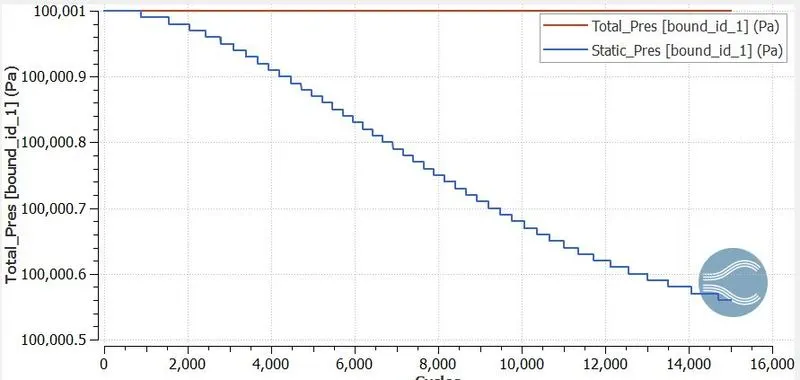
At the inlet the we observe that initially total and static pressure remains the same. As the cycles passes the static pressure is decreasing due the increase in dynamic pressure.
The total pressure is given as,
Total Pressure = Static Pressure+Dynamic Pressure.
After certain cycles we could observe that the static pressure decreases rapidly because of increase in speed of the fluid flow.
Total and Static Pressure at outlet:
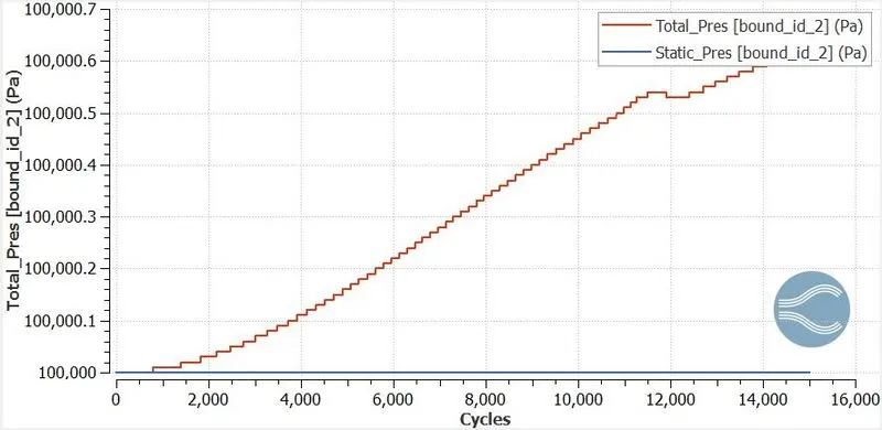
In the outlet the total pressure is increased because of the increase in dynamic pressure.
Mass Flow Rate:
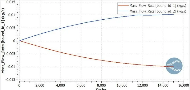
Mass flow rate is defined as the mass of the substance which passes per unit time. Here the mass flow rate at the inlet is decreased due to high pressure and low velocity.
Total Cell Count:
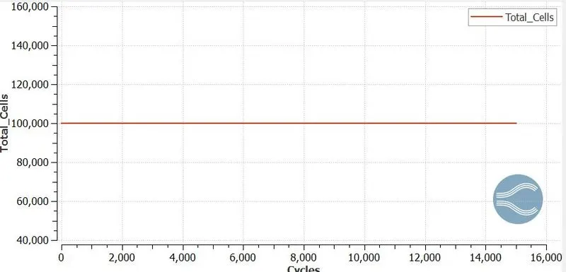
As we have fixed the mesh size to be 1.0e-4 there are total of 100000 cells created.
Rank0:
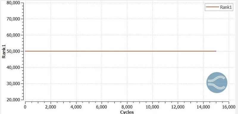
Rank1:
Animation for Case 3:
https://youtu.be/CfoIDLOfUcs
Conclusion:
- Thus in this challenge we have computed the 2D channel flow simulation using converge CFD by assigning different mesh size parameters in order to get more accurate and smooth results.
- Minimum time is consumed with low grid resolution but it provides the results with less accuracy and smoothness. In order to get results with high accuracy and smoothness it is best to choose the coarse mesh type but it consumes a lot of time.
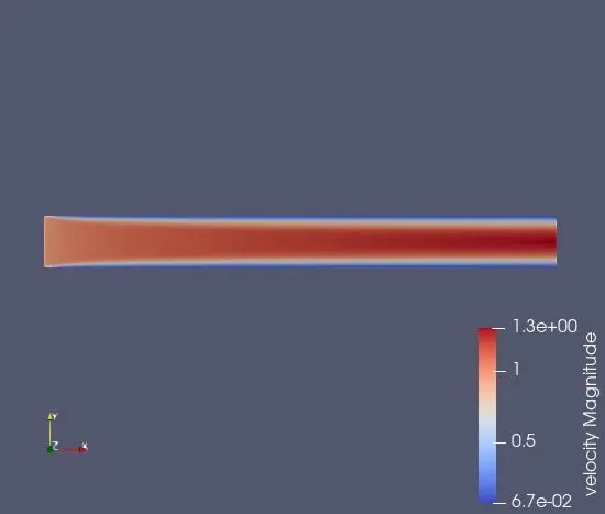
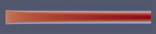
- From the contour plots we could observe that the flow velocity remains high at the centre of the channel and the flow velocity reduces near the wall because of the wall surface shear stress.
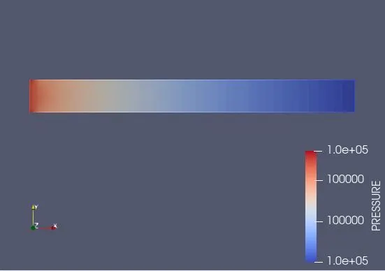
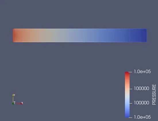
- From the pressure contour we could observe that the pressure is high at the starting of the flow and reduces constantly through out the flow through the channel.
- From the observation of the entire contour plots we could observe that each simulation is providing almost the same plot only change in result contour is their resolution. The fine grid gives a smooth flow contour than the coarse grid but with the a fine grid the computation time increases.