Week 1: Channel flow simulation using CONVERGE CFD

AIM:

(i) To Setup a simulation on the Channel Flow for three different meshes

(ii)To study about the parameters such as Pressure, Velocity, Mass Flow Rate for three different meshes with help of contours, Plots.

(iii)To understand the flow development with the help of animation

Introduction:

A substance in the liquid or gas phase is referred to as a fluid. Distinction between a solid and a fluid is made on the basis of the substance’s ability to resist an applied shear (or tangential) stress that tends to change its shape. A solid can resist an applied shear stress by deforming, whereas a fluid deforms continuously under the influence of a shear stress, (i) Fluids for which the rate of deformation is linearly proportional to the shear stress are called Newtonian fluids after Sir Isaac Newton, who expressed it first in 1687. Most common fluids such as water, air, gasoline, and oils are Newtonian fluids, (ii) For non-Newtonian fluids, the relationship between shear stress and rate of deformation is not linear. The slope of the curve on the 𝜏 versus chart is referred to as the apparent viscosity of the fluid (a) Fluids for which the apparent viscosity increases with the rate of deformation (such as solutions with suspended starch or sand) are referred to as dilatant or shear thickening fluid ,(b) the fluid becoming less viscous as it is sheared harder, such as some paints, polymer solutions, and fluids with suspended particles are referred to as pseudoplastic or shear thinning fluids. (c) Some materials such as toothpaste can resist a finite shear stress and thus behave as a solid, but deform continuously when the shear stress exceeds the yield stress and behave as a fluid. Such materials are referred to as Bingham plastics after Eugene C. Bingham (1878–1945) (d) Thixotropic liquids, that become less viscous over time when shaken, agitated, or otherwise stressed. Common examples include ketchup, paint, and certain gels. (e) Rheopectic liquids, that become more viscous over time when shaken, agitated, or otherwise stressed. Examples include some creams and gypsum paste

Flow are classified as (i) Viscous vs Inviscid Flows-Flows in which the frictional effects are significant are called viscous flows. Viscous forces are negligibly small compared to inertial or pressure forces. Neglecting the viscous terms in such inviscid flows.(ii)Internal vs External Flows-The flow in a pipe or duct is internal flow if the fluid is bounded by solid surfaces. Internal flows are dominated by the influence of viscosity throughout the flow field. The flow of an unbounded fluid over a surface such as a plate, a wire, or a pipe is external flow. In external flows the viscous effects are limited to boundary layers near solid surfaces and to wake regions downstream of bodies. The flow of liquids in a duct is called open-channel flow if the duct is only partially filled with the liquid and there is a free surface, (iii)Compressible vs Incompressible Flows-Liquid flows are incompressible to a high level of accuracy, but the level of variation of density in gas flows and the consequent level of approximation made when modeling gas flows as incompressible depends on the Mach number. Gas flows can often be approximated as incompressible if the density changes are under about 5 percent, which is usually the case when Ma < 0.3.Gas flows is compressible when density changes more than 5 percent, Mach number Ma > 0.3 ,(iv)Laminar vs Turbulent Flows-The highly ordered fluid motion characterized by smooth layers of fluid is called laminar. The highly disordered fluid motion that typically occurs at high velocities and is characterized by velocity fluctuations is called turbulent. Based on Reynolds number flow will characterize whether flow is laminar or turbulent.(v)Natural vs Forced Flow-In natural flows, fluid motion is due to natural means such as the buoyancy effect, which manifests itself as the rise of warmer (and thus lighter) fluid and the fall of cooler (and thus denser) fluid. In forced flow, a fluid is forced to flow over a surface or in a pipe by external means such as a pump or a fan.(vi)Steady vs Unsteady Flow-The term steady implies no change of properties, velocity, temperature, etc., at a point with time. The term Unsteady implies change of properties, velocity, temperature, etc., at a point with time. Unsteady is the most general term that applies to any flow that is not steady, but transient is typically used for developing flows.(vii)One-, Two-, and Three-Dimensional Flows-A flow field is best characterized by its velocity distribution, and thus a flow is said to be one-, two-, or three-dimensional if the flow velocity varies in one, two, or three primary dimensions, respectively. A typical fluid flow involves a three-dimensional geometry, and the velocity may vary in all three dimensions, rendering the flow three-dimensional [V›(x, y, z) in rectangular or V›(r, θ, z) in cylindrical coordinates]. However, the variation of velocity in certain directions can be small relative to the variation in other directions and can be ignored with negligible error. In such cases, the flow can be modeled conveniently as being one- or two-dimensional, which is easier to analyze. (viii) Uniform vs Non-Uniform Flow-Uniform flow implies that all fluid properties, such as velocity, pressure, temperature, etc., do not vary with position. Non-Uniform flow implies that all fluid properties, such as velocity, pressure, temperature, etc., vary with position.

Fluid mechanics is defined as the science that deals with the behavior of fluids at rest (fluid statics) or in motion (fluid dynamics), and the interaction of fluids with solids or other fluids at the boundaries(Fluid-Structure Interaction(FSI)).Branches of fluid mechanics are (i)The study of the motion of fluids that can be approximated as incompressible (such as liquids, especially water, and gases at low speeds) is usually referred to as Hydrodynamics. (ii) Hydraulics, which deals with liquid flows in pipes and open channels. (iii) Hydrology is the study of the distribution and movement of water both on and below the Earth's surface, as well as the impact of human activity on water availability and conditions.(iv) Gas dynamics deals with the flow of fluids that undergo significant density changes, such as the flow of gases through nozzles at high speeds.(v)Pneumatics is a branch of fluid mechanics that deals with the study and application of pressurized air and other gases. It involves using the pressure energy of compressed air to perform mechanical work. (vi) The category aerodynamics deals with the flow of gases (especially air) over bodies such as aircraft, rockets, and automobiles at high or low speeds (vii)Oceanography involves the study of Earth’s oceans, where fluid dynamics plays a key role in understanding complex patterns of fluid motion such as ocean currents, waves, and tides.

Theory:

Focusing on the airflow through the channels. Airflow, is the movement of air. The primary cause of airflow is the existence of air. Air behaves in a fluid manner, meaning particles naturally flow from areas of higher pressure to those where the pressure is lower. Atmospheric air pressure is directly related to altitude, temperature, and composition. Airflow is a measurement of the amount of air per unit of time that flows through a particular device. It can be described as a volumetric flow rate (volume of air per unit time) or a mass flow rate (mass of air per unit time). What relates both forms of description is the air density, which is a function of pressure and temperature through the ideal gas law. The flow of air can be induced through mechanical means (such as by operating an electric or manual fan) or can take place passively, as a function of pressure differentials present in the environment. Channel flow is an internal flow in which the confining walls change the hydrodynamic structure of the flow from an arbitrary state at the channel inlet to a certain state at the outlet. The simplest illustration of internal flow, Laminar flow in a circular tube (see Poiseuille Flow), while a turbulent flow in the rotor of a centrifugal compressor is an example of the most intricately-shaped internal flow (see Rotating Ducts). Engineering devices employ channels with cross-sections of various geometrical shapes. Some of the different types of channels based on cross-section are Rectangular channels, Trapezoidal channels, circular channels, Triangular Channels etc..., Noncircular pipes are usually used in applications such as the heating and cooling systems of buildings where the pressure difference is relatively small, the manufacturing and installation costs are lower, and the available space is limited for ductwork. Another name of closed Channels is Duct. In this, focus on the Rectangular Duct. Rectangular Duct geometry is defined as pipe of rectangular cross-section. The need for the hydraulic diameter arises due to the use of a single dimension in the case of a dimensionless quantity such as the Reynolds number, which prefers a single variable for flow analysis rather than the set of variables as listed in the table below. The Manning formula contains a quantity called the hydraulic radius. Despite what the name may suggest, the hydraulic diameter is not twice the hydraulic radius, but four times larger. Hydraulic diameter is mainly used for calculations involving turbulent flow. Secondary flows can be observed in non-circular ducts as a result of turbulent shear stress in the turbulent flow. Hydraulic diameter is also used in calculation of heat transfer in internal-flow problems. Hydraulic diameter is defined as the ratio of four times of area of cross-section of the flow to the wetted perimeter of the cross-section. Hydraulic Diameter is

-area of the cross section

-wetted perimeter

-hydraulic diameter.

Hydraulic diameter of the rectangular duct is given by

Area of rectangular cross-section-

-width of the cross section.

-Height of the cross section.

Wetted perimeter-

The fluid dynamics and heat transfer behavior of laminar and turbulent flow through noncircular ducts is of special interest because of the wide application of such geometries in compact heat exchangers. The usual boundary condition on the velocity for a fluid flowing through a noncircular channel is the relatively simple nonslip condition (i.e., the velocity goes to zero on the boundaries), the same as for circular pipe flow. However, the thermal boundary conditions encountered in noncircular duct flows are generally more complex than in the case of pipe flow. Unfortunately, noncircular ducts do not possess such symmetry and as a result there often exist peripheral variations in shear rate and shear stress as well as in temperature and heat flux, requiring simultaneous analysis of the conduction problem in the wall and the convection problem in the fluid.

Fluid flow through the Rectangular channel ,initially flow would be developing where gradients changes in the flow direction and for Developed flow where gradients doesn't change in flow direction. The analytical solution is also available for the fully developed laminar velocity profile of a Newtonian fluid in rectangular ducts

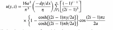
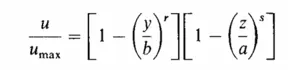
where r = 2 and s was obtained by applying the principle of minimum energy dissipation

Friction factors depends on the aspect ratio

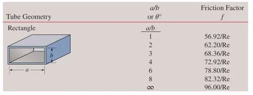
The pressure gradient in the region of flow development will differ from that of a fully developed flow. The length of the duct in which such a velocity development occurs is called the hydrodynamic entrance length or entrance region. The pressure decreases as a result of the wall shear and the change in momentum. The pressure drop in this region may be treated as consisting of two components: (1) the pressure drop based on the fully developed flow and (2) an additional pressure drop due to the momentum change and accumulated increment in wall shear between the developing flow and the developed flow

In the case of turbulent channel flow of Newtonian fluids, most of the resistance to the transfer of heat and momentum is concentrated in the laminar sublayer region near the wall. Accordingly, the temperature and velocity profiles are relatively flat over most of the cross section. Hence, the influence of duct shape in turbulent flow is generally not as great as in laminar flow. Therefore, it has been a common practice to estimate the friction factors and dimensionless heat transfer coefficients for noncircular ducts by using corresponding circular pipe results, replacing the diameter by the hydraulic diameter. The hydrodynamic entrance length of Newtonian fluids in turbulent duct flow is relatively short, generally not more than 10 to 20 hydraulic diameters. The thermal entrance region for turbulent duct flow of Newtonian fluids is relatively short, not more than 15 to 20 hydraulic diameters for various thermal boundary conditions. The following aspects are significant on turbulent flow they are (a) the Reynolds-number effect on secondary flow, (b) the directional characteristics of local wall shear stress, (c) the orientation of Reynolds-stress principal planes in a plane normal to the axial flow direction, and (d) the Reynolds equation along a secondary-flow streamline.

Case Setup:

1.Converge Studio Application is opened

Select New project

2.Create the channel geometry ,Geometry->create->shape->Box, after this, given inputs about center and the dx, dy, dz.

dx, dy, dz represents the length on the Each co-ordinate.

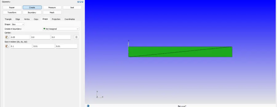
3.Geometry->Boundary->create a Boundary is selected, Creating multiple boundaries by selecting the checkbox on the Boundary Definition dialog box

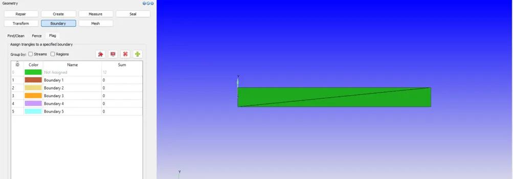
4.Renaming the created boundary by right-clicking the mouse. With the help of cursor pick selecting the entities and assigning to the boundary

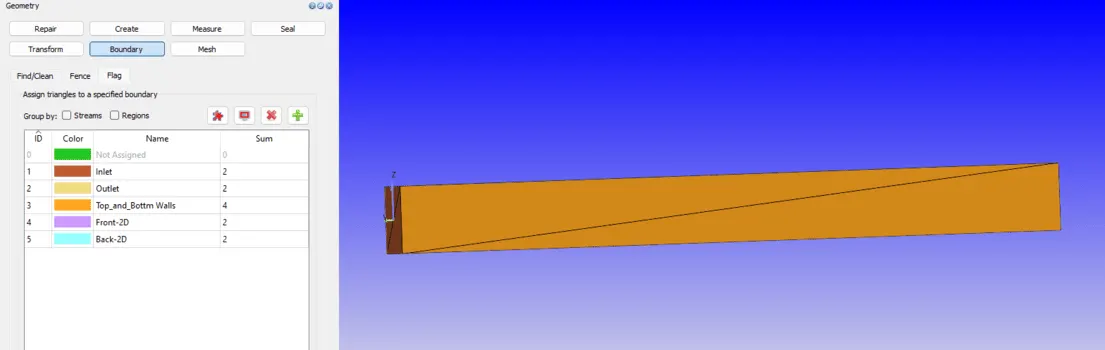
5.Selected Normal toggle will displays the surface normal. Geometry->transform->normal is selected then one of outward normal surface is selected and select propagate change from single face and then apply.

6.Click on the diagnosis tab to check the errors present in the model.

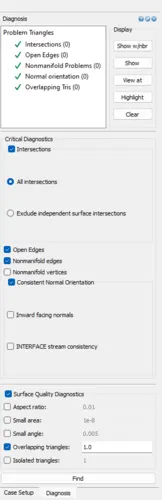
7.Click on case setup tab, then begin case setup is clicked to start the case setup

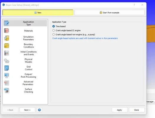
Selected a time-based.

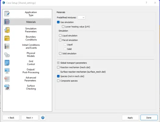
8.Selecting the materials, Predefined mixture as air, gas simulation and species is checked

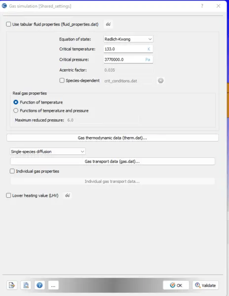
9.Gas simulation is selected then it provides a option to select the equation of state

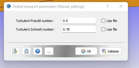
10.Global transport parameters is selected

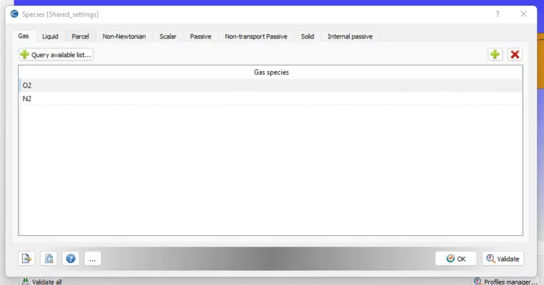
11.Selected the species then created the species on the species tab

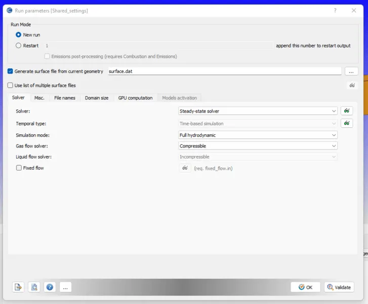
12.Select Run parameters then select the type of simulation as steady state

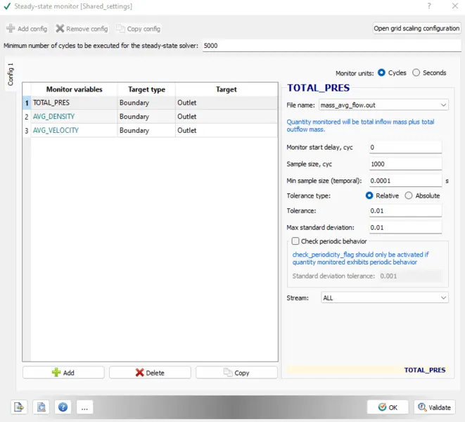
Select the steady state monitor and add config

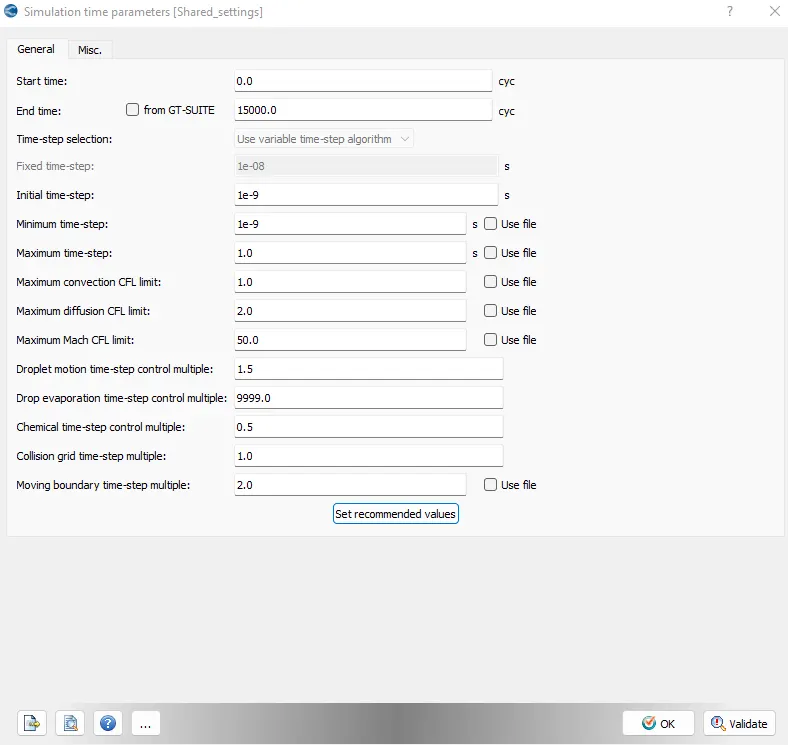
13.Select the simulation time parameter and choose the start time, end time, initial, min and max timestep, CFL limit ..

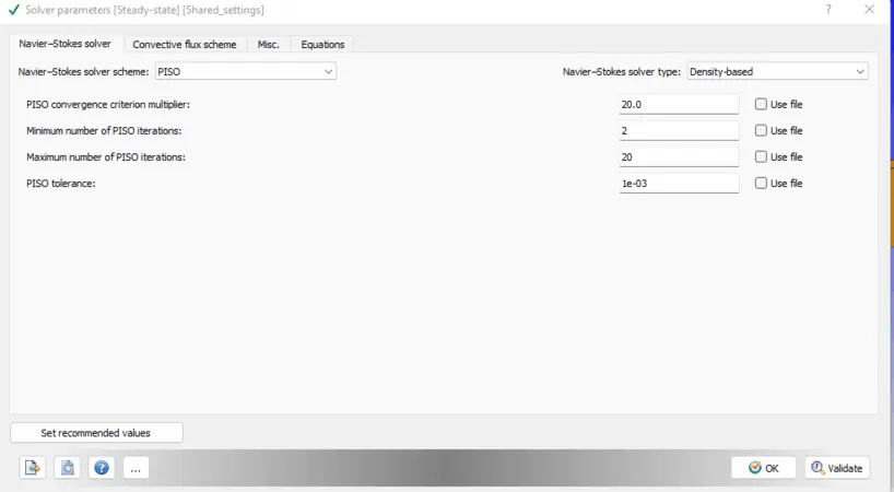
14.selecting the solver and the numerical schemes under the solver parameters.

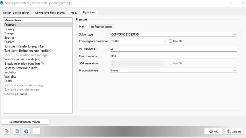
15.Defining the region

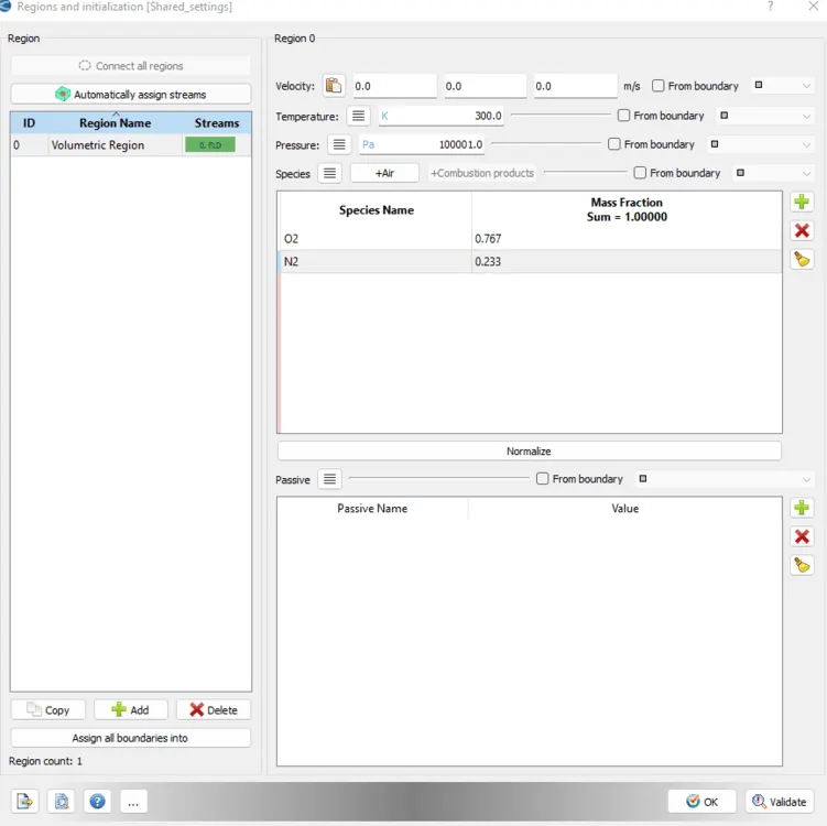
16.Defining the boundary by selecting the boundary conditions

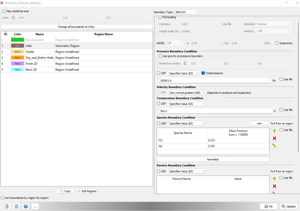
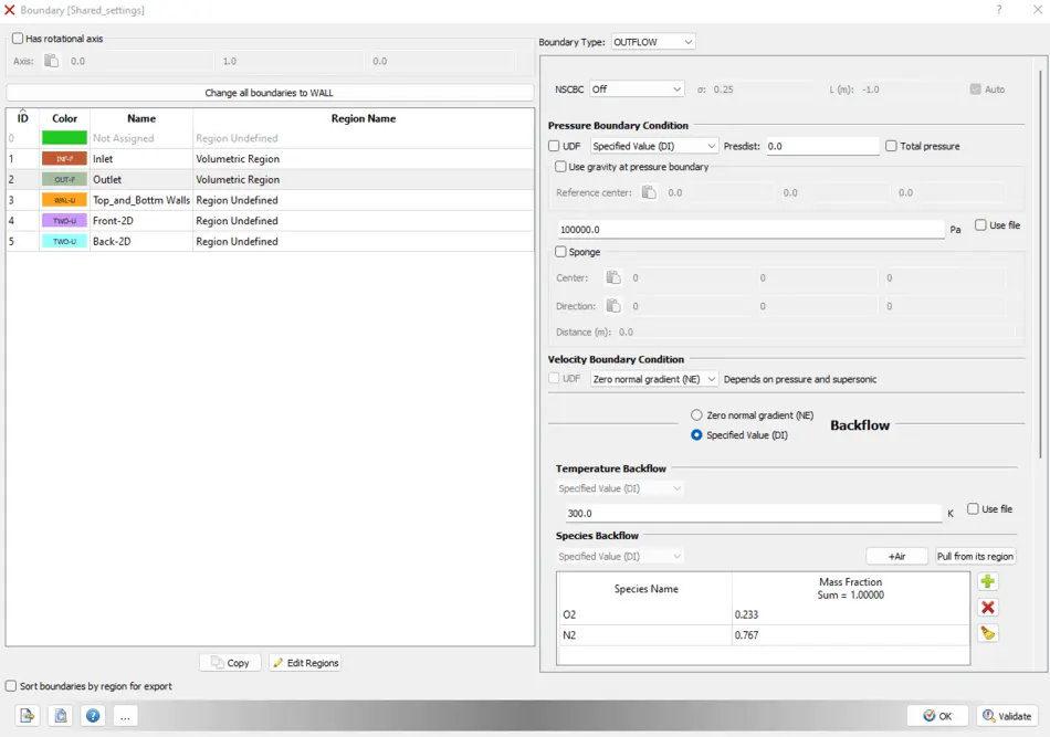
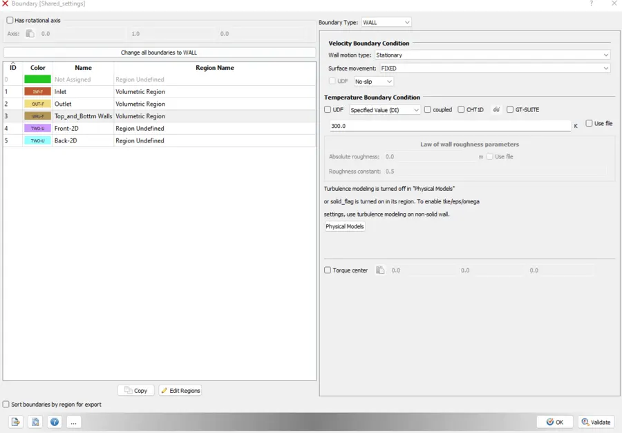
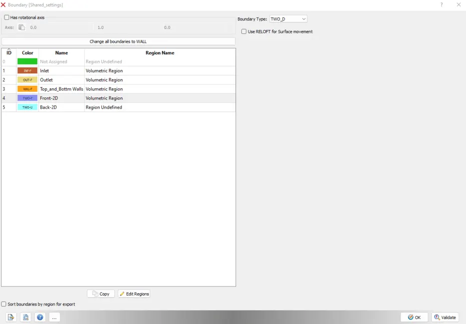
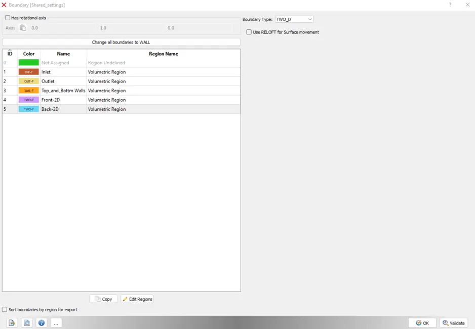
17.Not included any of the model so physical models consists only unchecked models. Laminar flow through the Channel

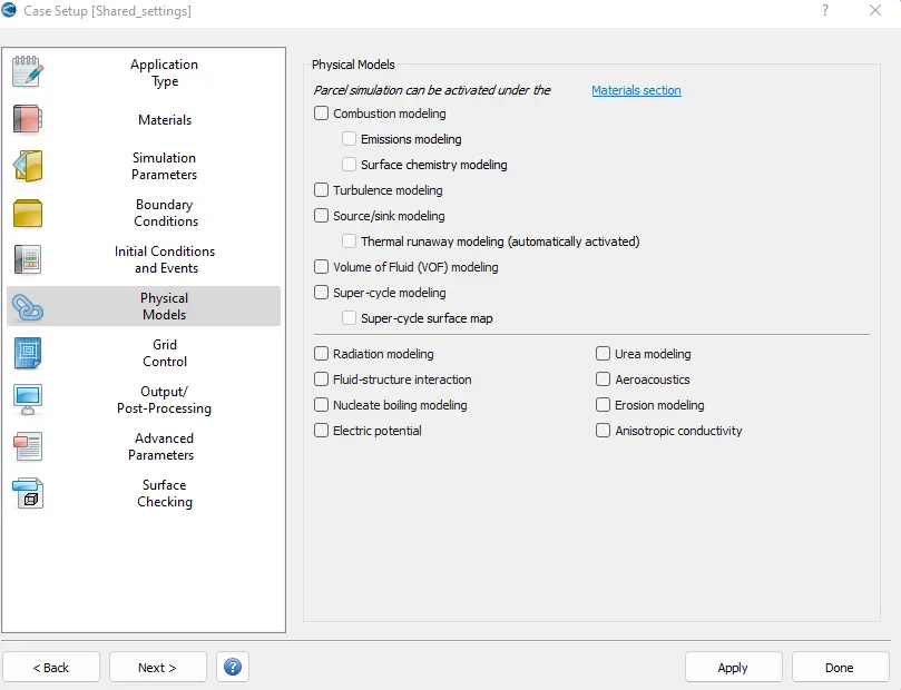
18.By selecting grid control can include an Adaptive Mesh Refinement

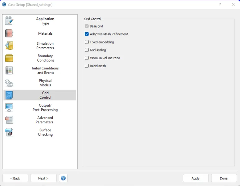
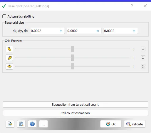
19.Base Grid is selected. To describe the grid length on each and every coordinates

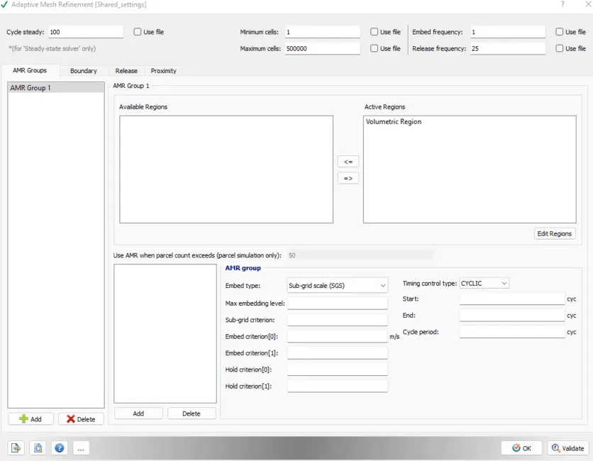
20.By Selecting Adaptive mesh refinement ,we can define maximum cells for the region

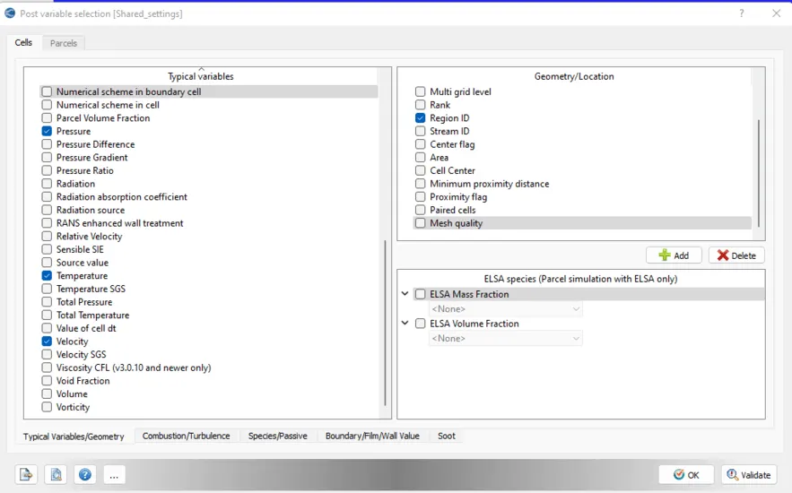
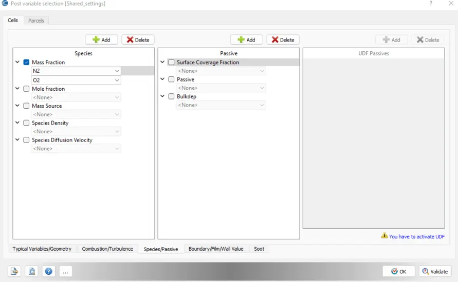
21.Selecting the post variable selection is used to select the variables, that is needed to post-process

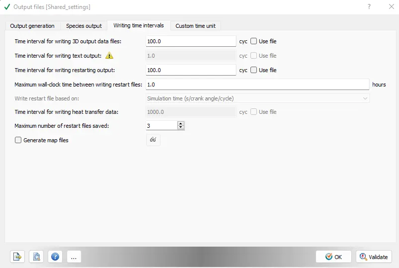
22.Output files has been selected, Maximum intervals of controlling output files.

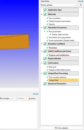
23.Final validating the case setup on the converge studio

24. Copying the executable files from Converge CFD installed folder to the location that consists the case setup files

25.cygwin terminal is navigated to the location consists a case setup files and then executed the code

mpiexec -n no.of.processors Executable_file --license file

26. Converting the 3D output files to Para View compatible file format with the help of post-processing 3D tab on the converge studio.

27. Load files onto the Para view to get the contours, velocity profiles, Animations etc...,

Mesh:

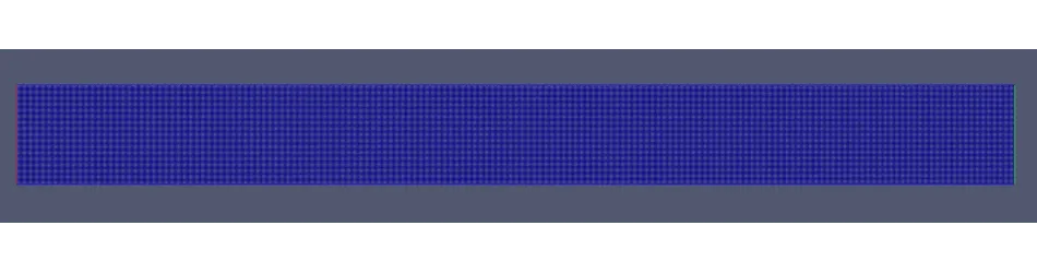
1.Base Mesh (Grid size-0.2 mm)

2.Medium Size Mesh (Grid Size-0.15 mm)

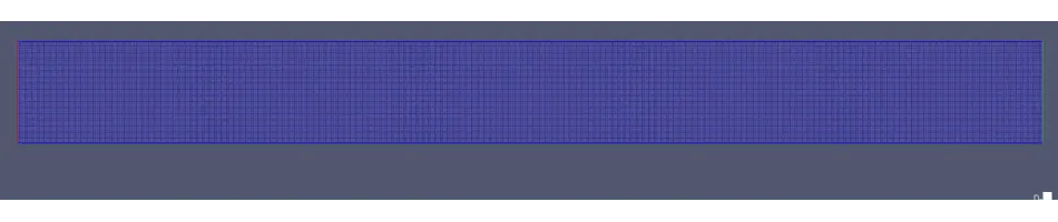
3.Fine Mesh (Grid Size-0.1 mm)

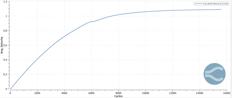
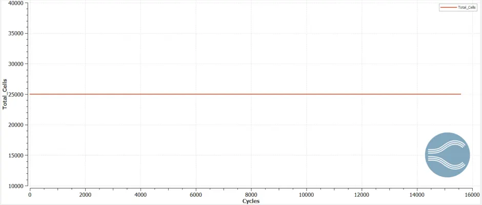
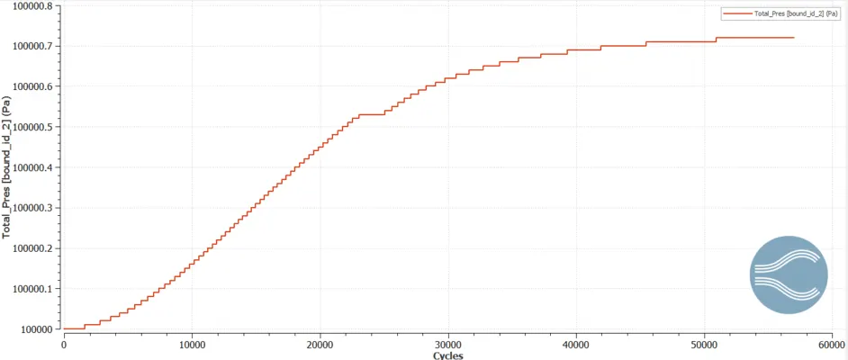
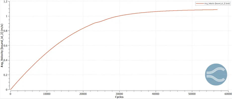
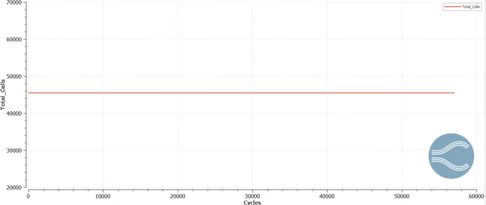
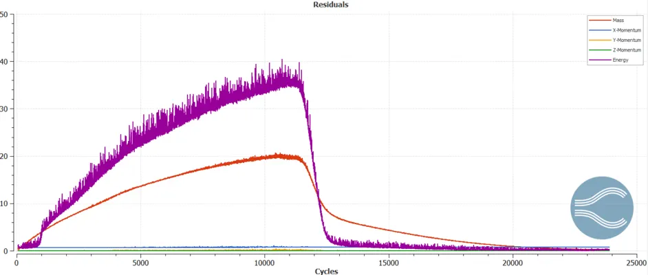
Monitor Plots:

Base Mesh

Medium Size Mesh:

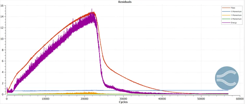
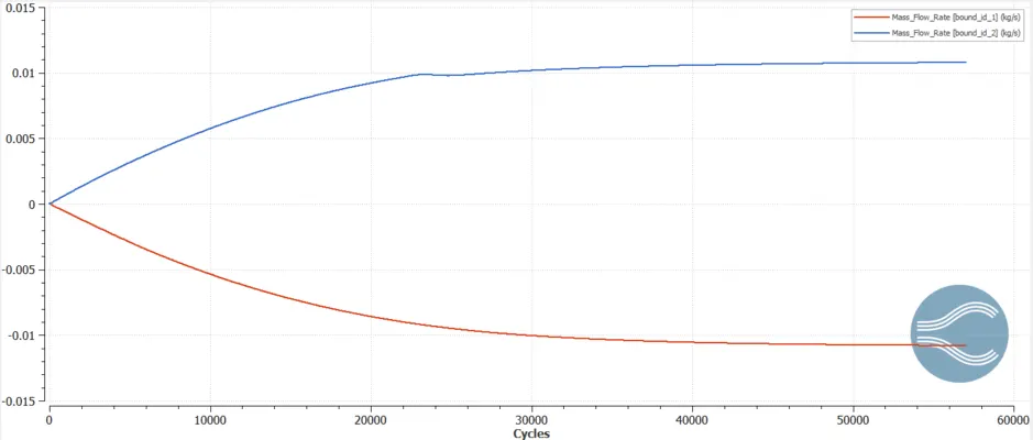
Fine Mesh:

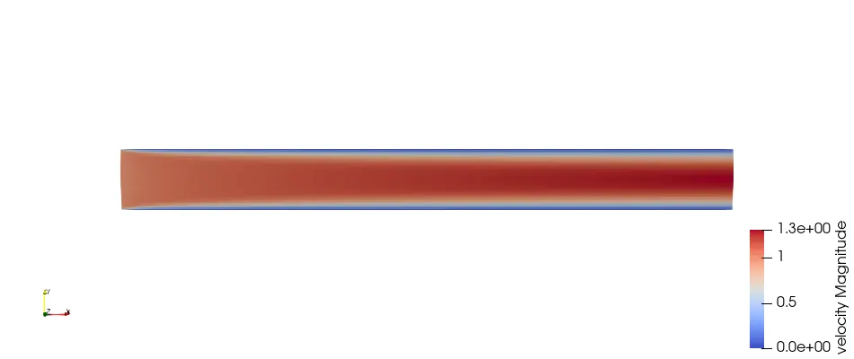
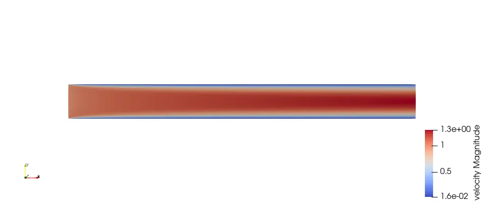
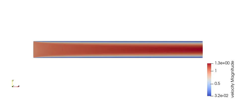
Velocity Contour:

Base Mesh

Medium size mesh

Fine Mesh

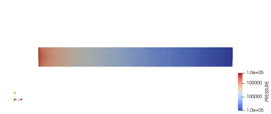
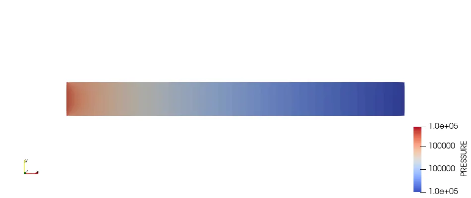
Pressure Contour:

Base mesh

Medium Size Mesh

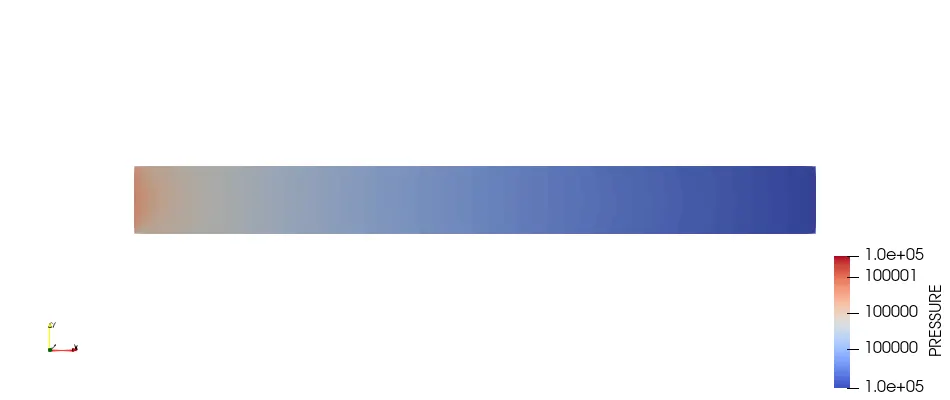
Fine Mesh

Conclusion:

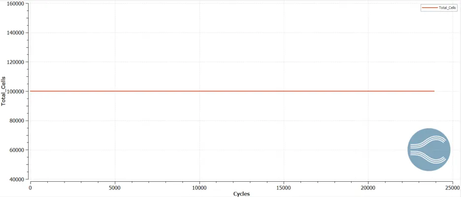
Cell counts for various grid sizes (i)0.2 mm grid size -25000 Cells (ii) 0.15 mm grid size-45420 cells (iii) 0.1 mm grid size-100000 cells

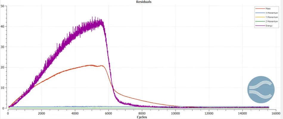
with the help of residual plots, observe base mesh(grid size-0.2 mm) has converged with less no of cycles

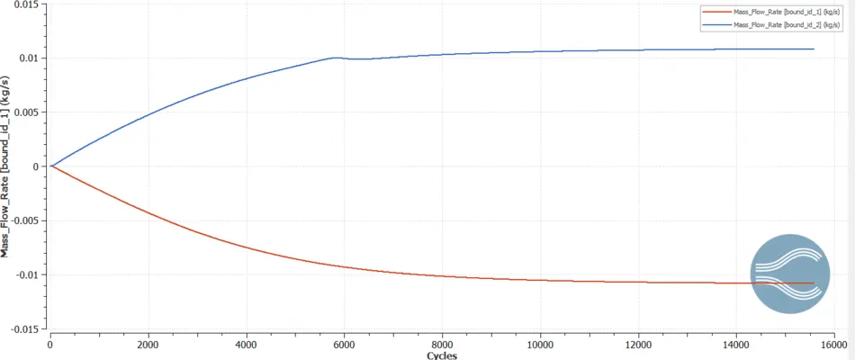
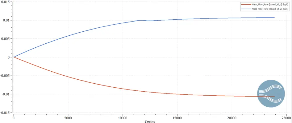
Mass flow rate plots help us to understand that inlet with negative quantity and outlet with positive quantity. The sum of inlet and outlet flow rate will give you net flow rate. Net mass flow rate for both base and medium mesh is conserved in the order of . But on the fine mesh the net mass flow rate in terms

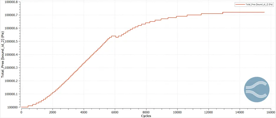
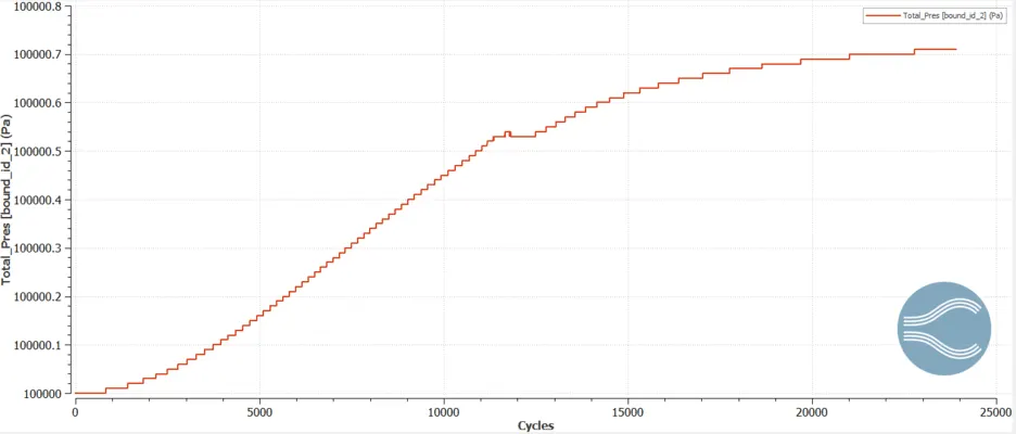
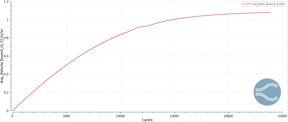
Average Velocity, Total pressure plots are increasing on the graph with increase of cycles

Velocity Contour does not show huge differences over the maximum value but it shows a differences of the minimum values of the contour

Total pressure plots does not show a difference ,even for three grid sizes.

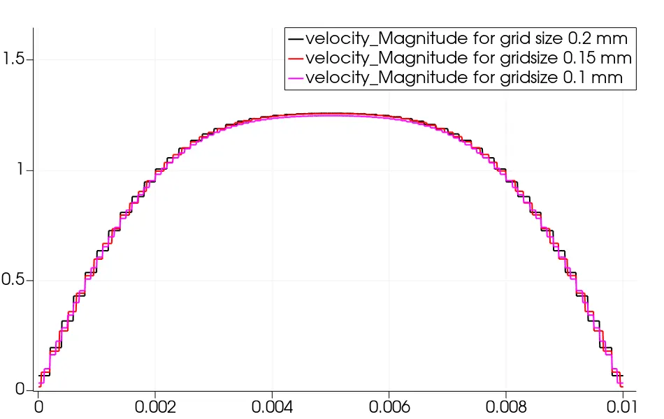
Velocity profiles for three grid sizes shown on the figure above. It doesn't show much differences on the velocity profiles

Maximum velocity for various grid Sizes (i)Grid size -0.2 mm, max velocity-1.258 m/s (ii)Grid size -0.15 mm, max Velocity-1.256 m/s (iii)Grid Size -0.1 mm, max Velocity-1.247 m/s. Change in max velocity is less than 1% for different grid sizes.

on the Fine Mesh, obtained the velocity profiles at the different lengths of the channel flow

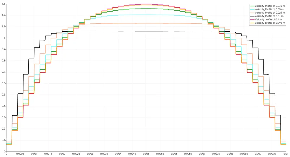
This plot indicates the derivative of the velocity with respect to the length in the flow direction is not zero.It show developing flow through the channel

A parabolic plot indicates the velocity profile of the laminar flow. Because of this, secondary flow cannot be able to observe, it is essential for the turbulent flow on the channels.

An Animation will used to study how the solver giving the results with respective to the cycles. So, the flow parameters such as pressure, velocity, etc..., will change from the initial values to the steady state results. It means flow is developing it starts with zero velocity, increase the velocity in the channel will show like fluid inside the channel is moving, reaches the steady state.

Base Mesh:https://youtu.be/cW5Tnzuqsgw

Medium size Mesh:https://youtu.be/GxSecQxgubM

Fine Mesh:https://youtu.be/pwhL73w-hrk