Week 1: Channel flow simulation using CONVERGE CFD

Aim: - To perform Channel Flow Simulation using Converge CFD.

Objective: -

1. To simulate channel flow and compare the result with 3 different base mesh sizes i.e.

dx = 2e-4 m dy = 2e-4 m dz = 2e-4 m

dx = 1.5e-4 m dy = 1.5e-4 m dz = 1.5e-4 m

dx = 1e-4 m dy = 1e-4 m dz = 1e-4 m

2. To plots for velocity, pressure, mass flow rate, and total cell count for all 3 base mesh sizes along with velocity and pressure contour.

Theory: -

Channel Flow –

Flow in which the fluid state is affected by a conduit or confining walls i.e., fluid enters at arbitrary state and exits at certain state is called Channel flow.

Channel flows are subdivided into two categories –

1. Open Channel Flow – These are flow in which there are free surface, for examples flow in rivers, irrigation canals etc.
2. Closed Conduit/Channel Flow – In these flows the fluid is confined in closed structure. It does not exert direct atmospheric pressure but hydraulic pressure on the walls of conduit. Its examples are pipe flow, flow through rectangular duct etc.

Not all flow within a closed conduit is considered pipe flow such as sewer systems in city where fluid flow with free surface hence, it is open channel low.

We are simulating Air Flow inside a Rectangular duct having dimensions length 10 cm and cross section area 1cm *1 cm. Three different mesh sizes are analyzed and compared to reach a more accurate conclusion.

For a developed and steady flow in rectangular duct for location (x,y,z) and velocity V(u,v,w) where x and u represent length and velocity along length respectively.

v=0, w= 0 and u = f (y,z)

w can be expressed in terms of differential equation:

`(∂^2u)/(∂y^2 ) + (∂^2u)/(∂z^2 ) =1/μ (∂p)/(∂x) =c`

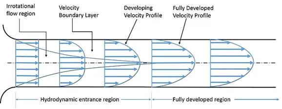
The developed flow is parabolic in nature and fully develop after certain length in the duct known as entrance length.

Case Setup: -

1. A box is created of length 10 cm and width and height 1 cm each with center at 5 cm and appropriate regions are defined as below:

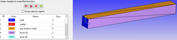
Normal of the boundary should point toward Fluid, hence normal are transformed accordingly.

2. A time base application type simulation with turbulence model off.

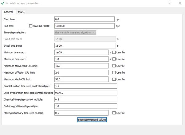
3. The solution run for 15000 cycles with minimum time step of 1e-9 s and maximum upto 1 sec.

4. Two species are selected which is predominant in Air i.e., O2 and N2.

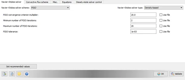
5. Steady state Solver with PISO scheme and since low pressure difference hence low Reynolds Number hence, pressure-based solver type is used.

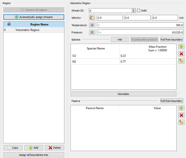
6. Volumetric Region are initialized with mass fraction of O2: 0.23 and N2: 0.77. The boundaries are assigned their region type.

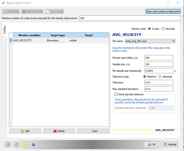
7. An average velocity monitor is set to monitor velocity during simulation.

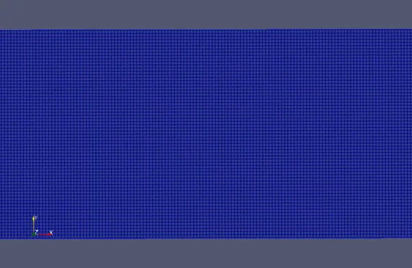
8. Grid size is given for all three directions and 3 base mesh are set which are simulated with same conditions. Mesh sizes are –

dx = 2e-4 m dy = 2e-4 m dz = 2e-4 m

dx = 1.5e-4 m dy = 1.5e-4 m dz = 1.5e-4 m

dx = 1e-4 m dy = 1e-4 m dz = 1e-4 m

9. The input files are exported to a folder to further solving.

Solving using Cygwin:

An executable “mpiexec.exe” is placed with the exported folder. The Cygwin directory is navigated to the above saved folder and following code is entered to solve the problem.

"mpiexec.exe -n 2 "C:\Program Files\Convergent_Science\CONVERGE\3.0.16\bin\intelmpi\converge.exe" restricted </dev/null> logfile &"

where address in quotes gives the path of folder containing input file exported earlier.

Post-Processing:

Post-Processing is done with the help of Converge CFD post processing tab –

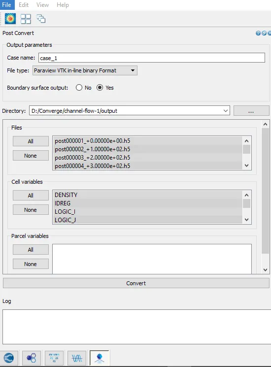
with these the output 3D data is converted in .vtm file and contours and animations are prepared though ParaView.

Results: -

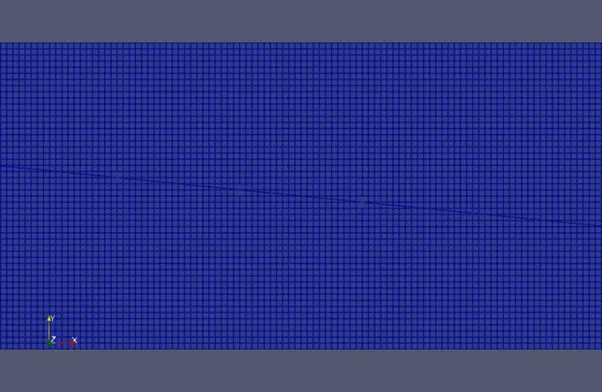
case 1: For mesh size = 2e-4 m

mesh:

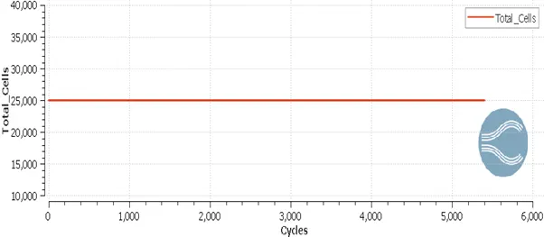
Total cell Count:

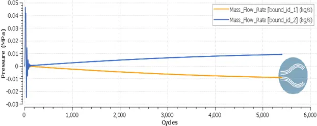
Mass Flow Rate: id_1 is inlet and id_2 is outlet

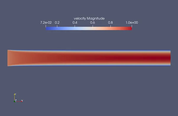
Velocity Contour:

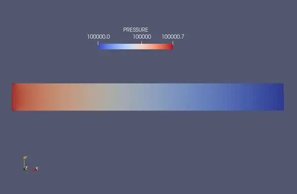
Pressure Contour:

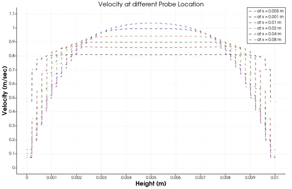
Velocity Profile at Different Line Probe Locations:

Velocity Animation:

case 2: For mesh size = 1.5e-4 m

mesh:

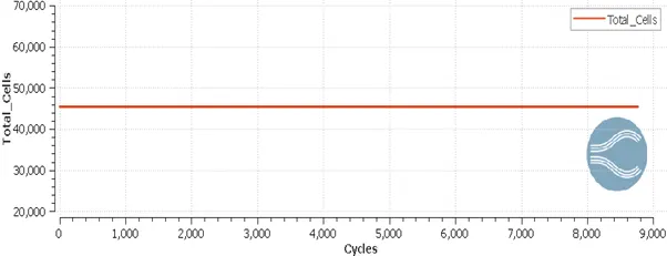
Total cell Count:

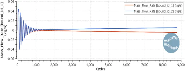
Mass Flow Rate: id_1 is inlet and id_2 is outlet

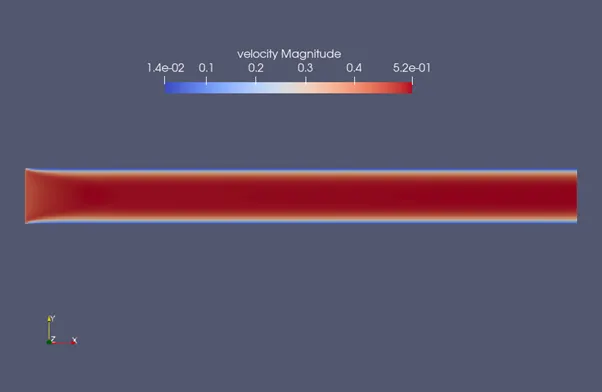
Velocity Contour:

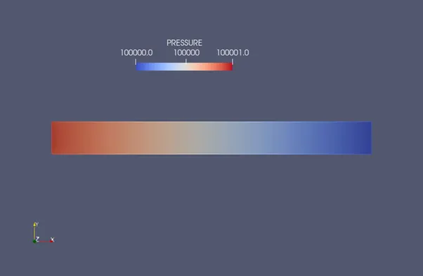
Pressure Contour:

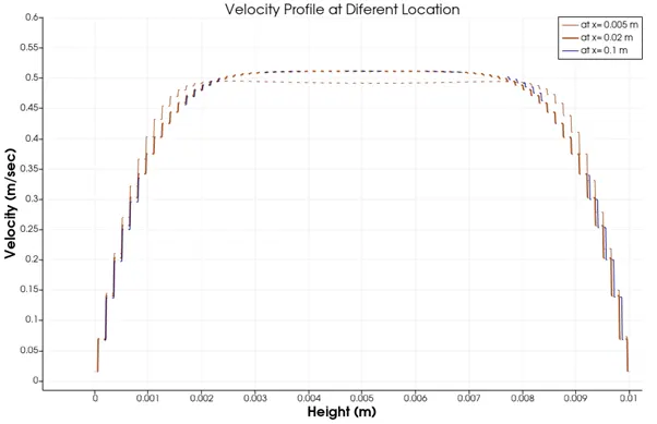
Velocity Profile at Different Line Probe Locations:

Velocity Animation:

case 3: For mesh size = 1e-4 m

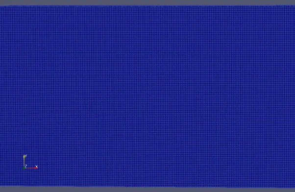
mesh:

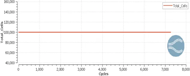
Total cell Count:

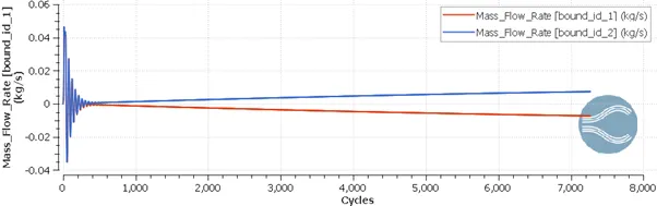
Mass Flow Rate: id_1 is inlet and id_2 is outlet

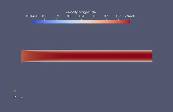
Velocity Contour:

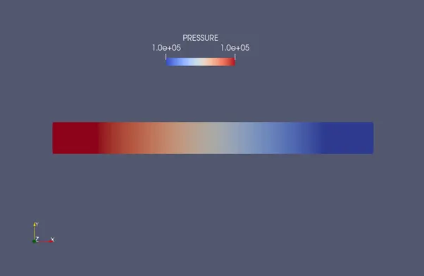
Pressure Contour:

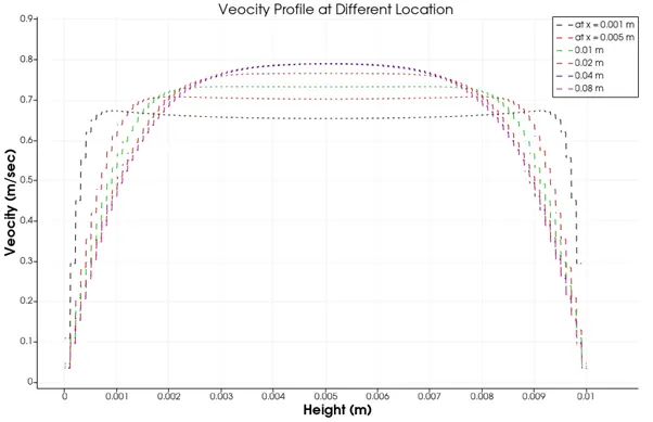
Velocity Profile at Different Line Probe Locations:

Velocity Animation:

Conclusion: -

1. Veocity Profile is more accurate for 1e-4 mesh size.

2. the mesh size 1.5e-4 produce less accurate resultcompared to other two and terminate after higher no. of cycles consuming more time.

3. 1e-4 mesh size produce better result as velocity profile is fully developed.

4. Decreasing the mesh size increses the result accuracy at expence of calculation time.