Channel flow simulation using CONVERGE CFD

Channel flow simulation using CONVERGE CFD

• Aim:

- Create a flow simulation of laminar flow in a channel

- Create a 2D simulation using the pressure inlet-outlet boundary conditions

- Generate the velocity profile and other parameters for 3 diffferent mesh sizes

• Theory:

1. Channel flow:

Channel flow, a branch of hydraulics and fluid mechanics, is a type of liquid flow within a conduit or in channel with a free surface, known as a channel. The other type of flow within a conduit is pipe flow. These two types of flow are similar in many ways but differ in one important respect: the free surface. Open-channel flow has a free surface, whereas pipe flow does not.

The behavior of open-channel flow is governed by the effects of viscosity and gravity relative to the inertial forces of the flow. Surface tension has a minor contribution, but does not play a significant enough role in most circumstances to be a governing factor. Due to the presence of a free surface, gravity is generally the most significant driver of open-channel flow; therefore, the ratio of inertial to gravity forces is the most important dimensionless parameter.

2. Laminar flow:

In fluid dynamics, laminar flow is characterized by fluid particles following smooth paths in layers, with each layer moving smoothly past the adjacent layers with little or no mixing.At low velocities, the fluid tends to flow without lateral mixing, and adjacent layers slide past one another like playing cards.

Here the flows are laminar due to the Pressure difference being very low from the inlet ot the outlet of the channel flow.

• Procedure:

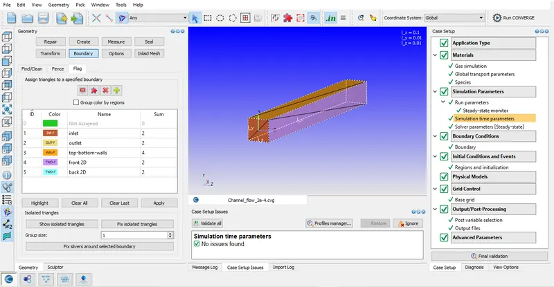
1. Create the 3D geometry using converge studio v3.0. Use the geometry tools to create a channel having dimensions of 0.1X0.01X0.01 and X having center at 0.05.

2. Assign boundary names appropriately and invert the normal facing outwards to inward since the fluid is present inside walls

3. Diagnose the geometry to check if there are any geomtery errors.

- Case Setup :

1. Application Type - Time-based

2. Materials -

a. Gas simulation- Air (predefined)

b. Global transport properties- Default settings

c. Species- O2 and N2 gases.

3. Simulation Parameters-

1. Run Parameters-

- Steady state solver, compressible, fully hydrodynamic

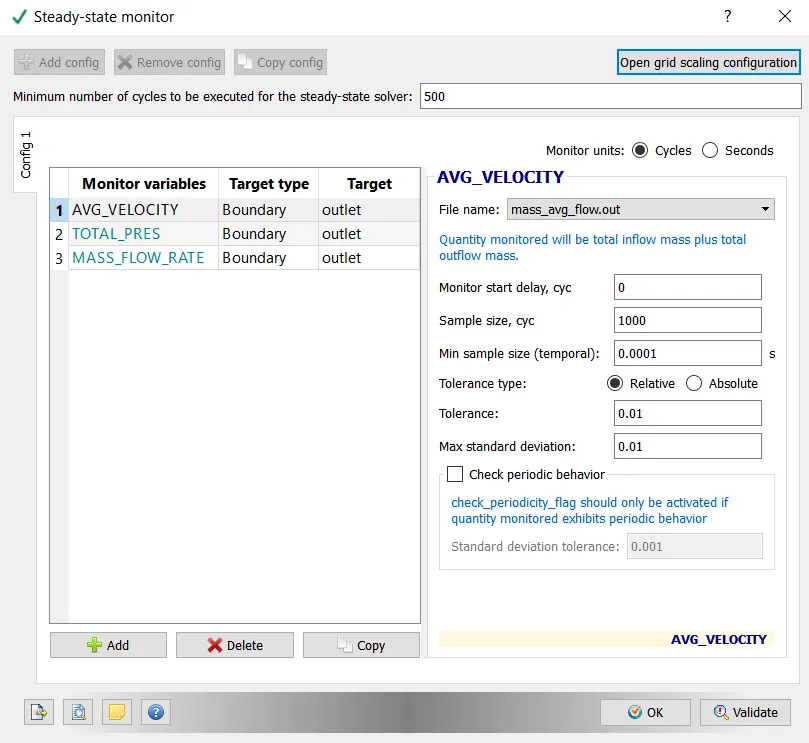
- Misc- choose steady state monitor and uncheck shared memory.

a. Steady-State Monitor-

2. Simulation Time Parameters:-

- End time- 15000 cycles

- Time step- 1e-9

- min time step- 1e-9

- max time step- 1

- Convection CFL number- 0.5

3. Solver Parameters [Steady-State]-

- Solver type- density based solver

- Equations- pressure- change preconditioner to none

- steady state solver control- convection CFL limit- 0.5

4. Boundary Conditions-

a. Inlet- Inflow

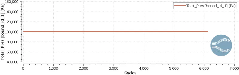
- Total pressure- 100001 Pa

- Initial temp- 300K

- Species boundary condition- add air

b. Outlet- Outflow

- Pressure- 100000 Pa

- Backflow - temp= 300k

- add air

c. Top-bottom-walls- Walls

no slip condition- The contact region between wall surface and fluid region tends to create high friction and create a 0 velocity of fluid flow, and due to viscosity of fluid, the fluid layers tend to undergo shear stress and have high pressure and overlap on eachother which eventually forms a fully developed region where velocity is max and constant and having low pressure.

d. Front and back wall: 2D- Since we are dealing with a 2D simulation the front and back regions can be considered as a symmetry or 2D wall condition.

5. Initial Conditions and Events:-

- Regions and Initialization:

Add air and Change the mass fraction of O2 to 0.77 and N2 to 0.23 so that we can notice the changes while post-processing and also even if the composition is different from the actual mole fractions of air, Converge still accepts the inputs and gives results according to its input. Therefore it can understand that the simulation takes place as long the case setup is correct and mole fraction sums up to 1.

6. Physical Models:-

Uncheck Turbulence Modeling in this case since we are dealing with laminar flows.

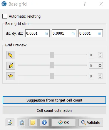
7. Grid Control:-

Base Grid:

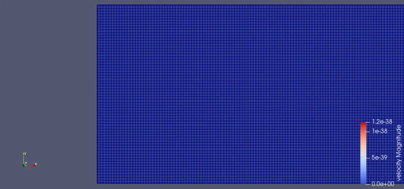
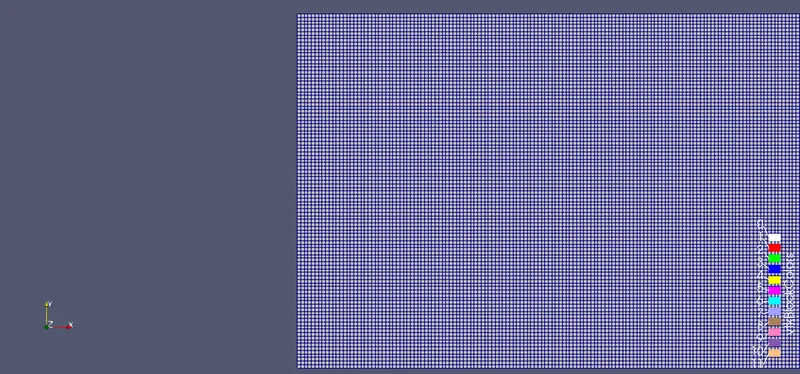
case-1, dx = 2e-4m, dy = 2e-4m, dz = 2e-4m

case-2, dx = 1.5e-4m, dy = 1.5e-4m, dz = 1.5e-4m

case-3, dx = 1.0e-4m, dy = 1.0e-4m, dz = 1.0e-4m

8. Post-Processing:-

- Post Variable Selection:

Select the parameters needed to be post processed. Unselect the turbulece parameters since we are interested in the turbulence modelling.

Select N2 and O2 in mole fraction under species

- Output files:

We need to set a time interval for the files to be saved during each set of iterations. It is best suited to have a min of 100 saved files for every simulation. Therefore we need to calculate the time interval for writing the output files based on our end time given in run parameters.

Restart files help in restoring the files if there is a sudden power cut/ crash which is not helpful or might end up loosing the entire data, therefore the restart files helps in resuming the simulation form the point we lost contact. Restart files time interval can be same as the writing files interval which is safe and healthy.

In this case- since the end time is 15000, we can have a time interval of 150 and the total files created will be 100.

• Results:

1. Mesh grid of 3 different mesh sizes:

a. 2e-4:

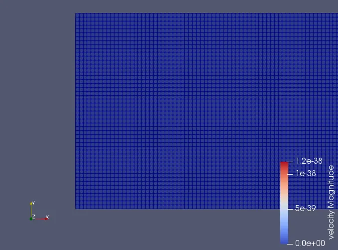
b. 1.5e-4:

c. 1e-4:

Discussion:

- Mesh is more finer as the distance between each cell is refined, this inturn results in accurate results but also requires more computational time and stability of the simulation reduces due to the CFL condition.

- The Navier stokes equation is solved for each cell depend upon different discreatisation schemes used to solve the domain.

2. Results for grid size 2e-4:

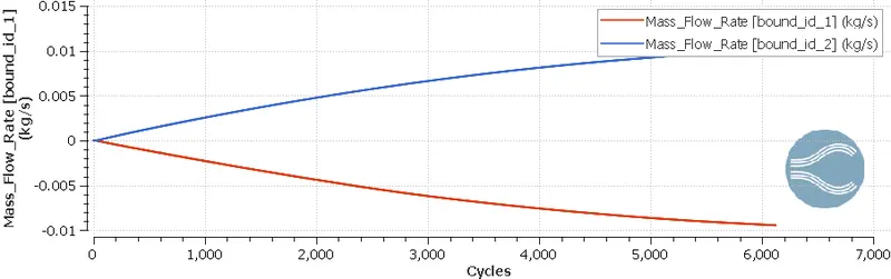
a. Mass flow rate at inlet and outlet:

b. Total pressure at inlet and outlet:

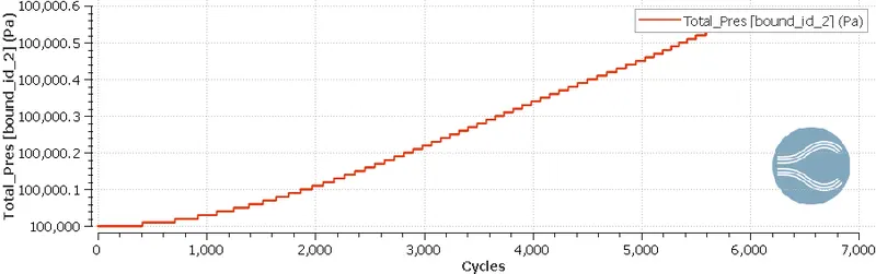
c. Static pressure at inlet and outlet:

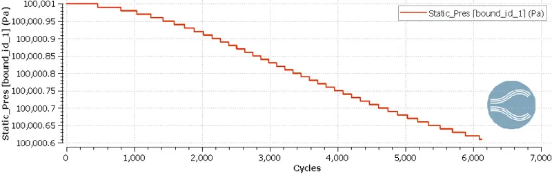
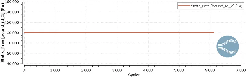
d. Average velocity at inlet and outlet:

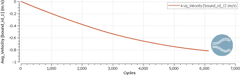
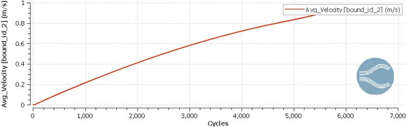
- Plot over line along and across flow direction:

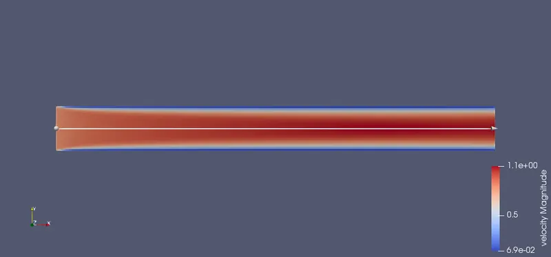
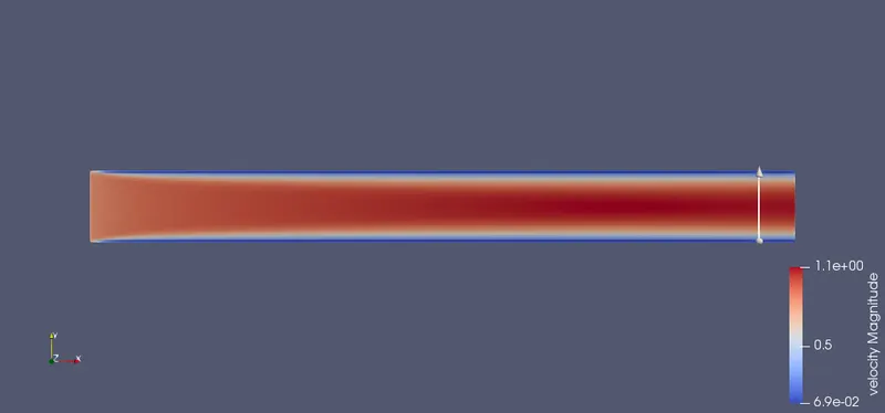
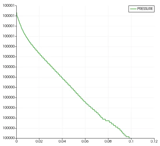
e. Pressure along the flow:

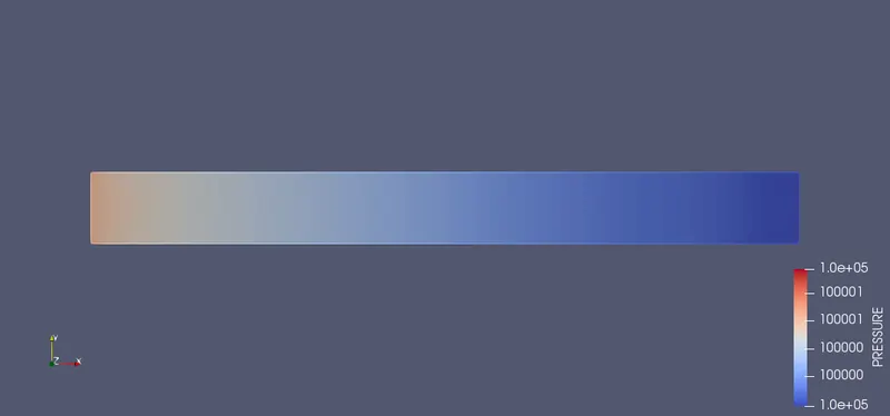
f. Velocity along the flow direction:

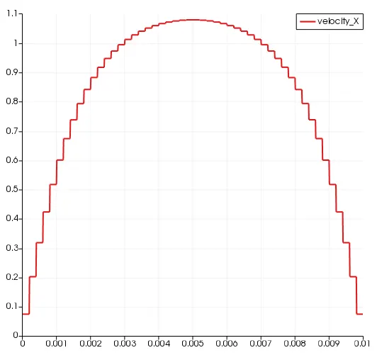
g. Velocity across the flow direction after fully developed region:

h. Flow animation clip:

3. Results for grid size 1.5e-4:

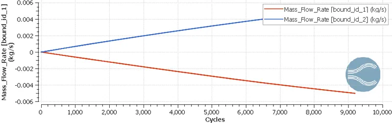
a. Mass flow rate:

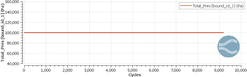
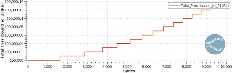
b. Total pressure at inlet and outlet:

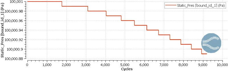
c. Static pressure at inlet and outlet:

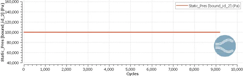
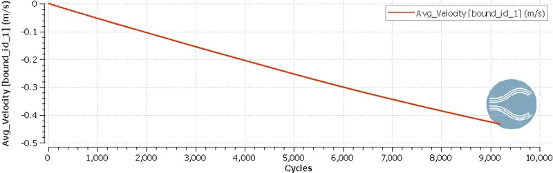
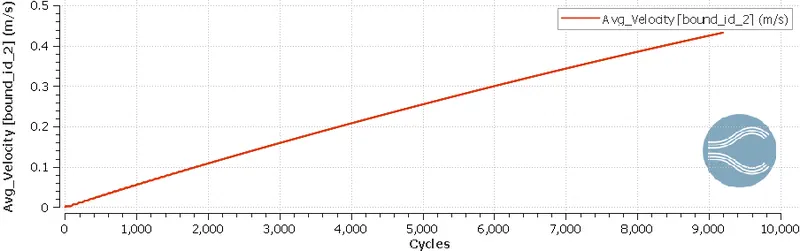
d. Average velocity at inelt and outlet:

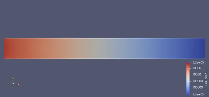
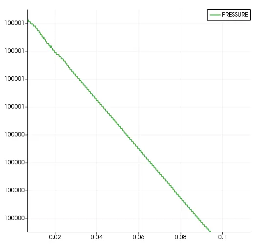
e. Pressure along the flow:

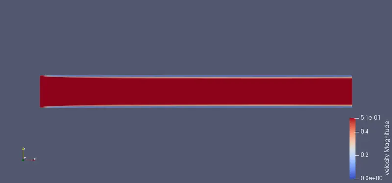
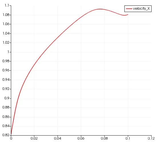
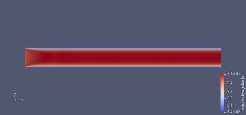
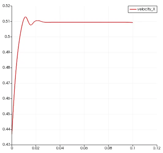
f. Velocity along the flow direction:

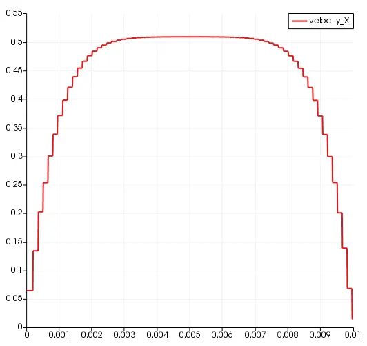
g. Velocity profile across flow direction after fully developed region:

h. Flow animation:

4. Results for grid size 1e-4:

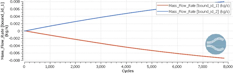
a. Mass flow rate:

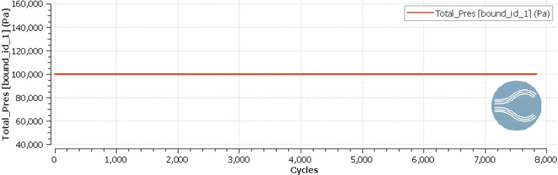
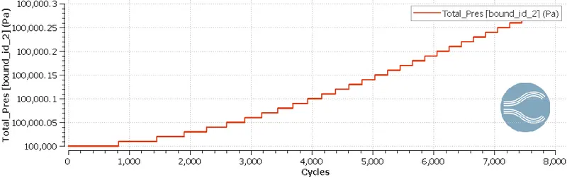
b. Total pressure at inlet and outlet:

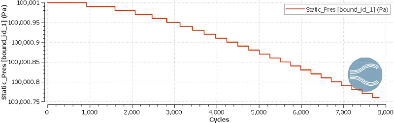
c. Static pressure at inlet and outlet:

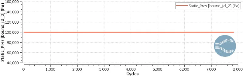
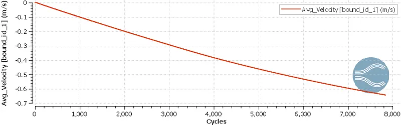
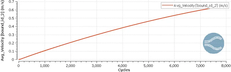
d. Average velocity at inlet and outlet:

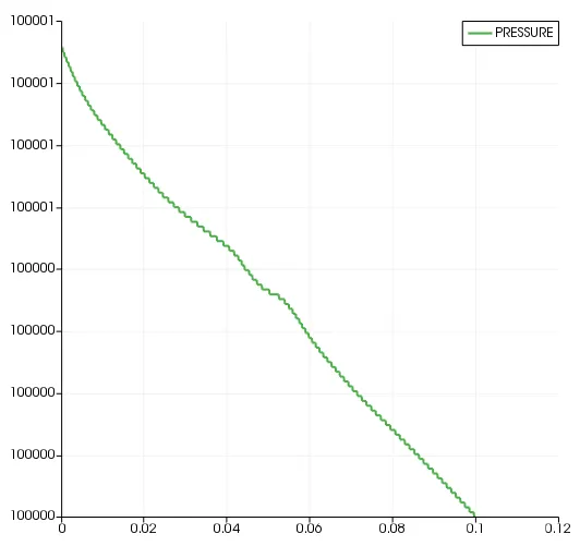
e. Pressure along the flow direction:

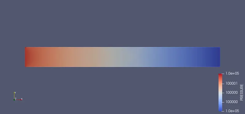
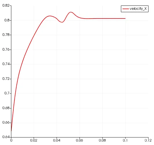
f. Velocity along the flow direction:

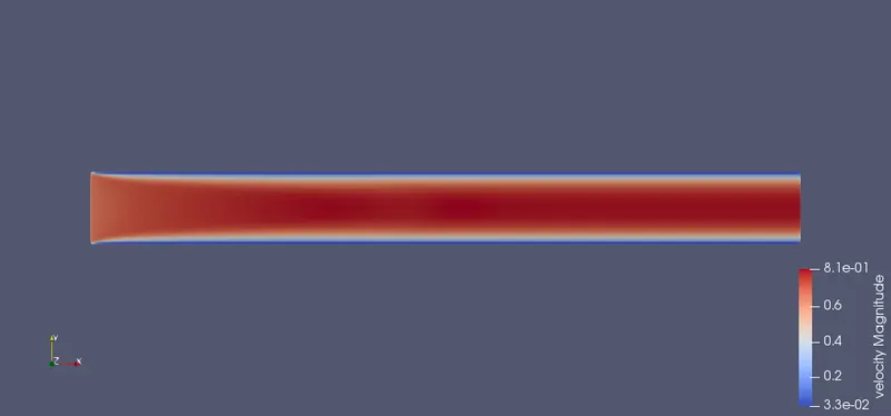
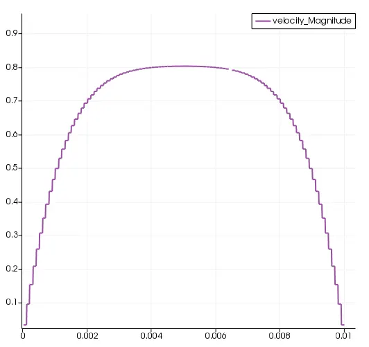
g. Velocity profile across the fluid flow after the fully developed region:

h. Flow animation:

• Discussions:

1. The Fully developed fluid flow is achieved at the outlet having max velocity and low pressure.

2. As the mesh is refined, the accuracy of the simulation is much greater but the stability.

3. Since the pressure difference is of 0.1 Bar, the velocity change is low and the flow tends to be laminar flow.

4. Since we are interested in the flow physics independent of time, we haved consider a steady-state simulation. therefore, turbulence modelling is avoided.

5. Due to the simple nature of the problem, the simulation time taken is quite low and convergence is reached at lesser iterations.

6. Mass flow rates are conserved and the plots of velocity and pressure along the fluid flow direction satisfy the general physics and is true in nature which helps in validating the problem.

7. Velocity profile created at the fully developed region across the fluid flow gives us a parabolic plot stating that the velocities of fluid are 0 at the wall due to high friction and viscocities. Pressure is high at the walls and lowest at the center of the flow and velocities are 0 at the wall and highest at the center of fluid flow.